The modified version of lightweight coreset for scalable \(k\)-means computation is applied for manifold-valued data \(X_1,X_2,\ldots,X_N \in \mathcal{M}\). The smaller the set is, the faster the execution becomes with potentially larger quantization errors.
Arguments
- riemobj
a S3
"riemdata"class for \(N\) manifold-valued data.- k
the number of clusters.
- M
the size of coreset (default: \(N/2\)).
- geometry
(case-insensitive) name of geometry; either geodesic (
"intrinsic") or embedded ("extrinsic") geometry.- ...
extra parameters including
- maxiter
maximum number of iterations to be run (default:50).
- nstart
the number of random starts (default: 5).
Value
a named list containing
- cluster
a length-\(N\) vector of class labels (from \(1:k\)).
- means
a 3d array where each slice along 3rd dimension is a matrix representation of class mean.
- score
within-cluster sum of squares (WCSS).
References
Bachem O, Lucic M, Krause A (2018). “Scalable k -Means Clustering via Lightweight Coresets.” In Proceedings of the 24th ACM SIGKDD International Conference on Knowledge Discovery & Data Mining, 1119–1127. ISBN 978-1-4503-5552-0.
Examples
#-------------------------------------------------------------------
# Example on Sphere : a dataset with three types
#
# class 1 : 10 perturbed data points near (1,0,0) on S^2 in R^3
# class 2 : 10 perturbed data points near (0,1,0) on S^2 in R^3
# class 3 : 10 perturbed data points near (0,0,1) on S^2 in R^3
#-------------------------------------------------------------------
## GENERATE DATA
mydata = list()
for (i in 1:10){
tgt = c(1, stats::rnorm(2, sd=0.1))
mydata[[i]] = tgt/sqrt(sum(tgt^2))
}
for (i in 11:20){
tgt = c(rnorm(1,sd=0.1),1,rnorm(1,sd=0.1))
mydata[[i]] = tgt/sqrt(sum(tgt^2))
}
for (i in 21:30){
tgt = c(stats::rnorm(2, sd=0.1), 1)
mydata[[i]] = tgt/sqrt(sum(tgt^2))
}
myriem = wrap.sphere(mydata)
mylabs = rep(c(1,2,3), each=10)
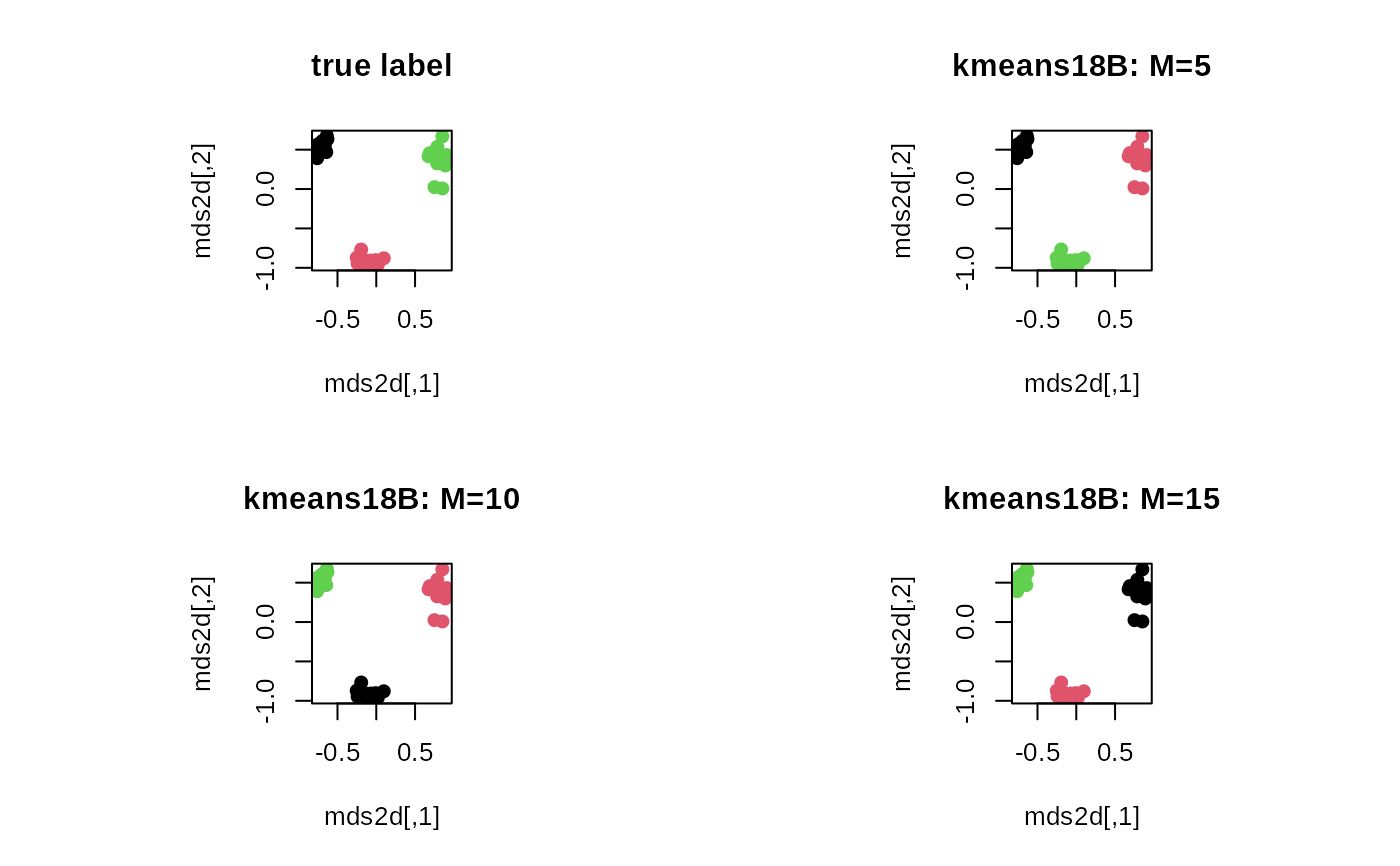
## TRY DIFFERENT SIZES OF CORESET WITH K=4 FIXED
core1 = riem.kmeans18B(myriem, k=3, M=5)
core2 = riem.kmeans18B(myriem, k=3, M=10)
core3 = riem.kmeans18B(myriem, k=3, M=15)
## MDS FOR VISUALIZATION
mds2d = riem.mds(myriem, ndim=2)$embed
## VISUALIZE
opar <- par(no.readonly=TRUE)
par(mfrow=c(2,2), pty="s")
plot(mds2d, pch=19, main="true label", col=mylabs)
plot(mds2d, pch=19, main="kmeans18B: M=5", col=core1$cluster)
plot(mds2d, pch=19, main="kmeans18B: M=10", col=core2$cluster)
plot(mds2d, pch=19, main="kmeans18B: M=15", col=core3$cluster)
 par(opar)