Given \(N\) observations \(X_1, X_2, \ldots, X_N \in \mathcal{M}\), perform k-means clustering by minimizing within-cluster sum of squares (WCSS). Since the problem is NP-hard and sensitive to the initialization, we provide an option with multiple starts and return the best result with respect to WCSS.
Usage
riem.kmeans(riemobj, k = 2, geometry = c("intrinsic", "extrinsic"), ...)Arguments
- riemobj
a S3
"riemdata"class for \(N\) manifold-valued data.- k
the number of clusters.
- geometry
(case-insensitive) name of geometry; either geodesic (
"intrinsic") or embedded ("extrinsic") geometry.- ...
extra parameters including
- algorithm
(case-insensitive) name of an algorithm;
"MacQueen"(default), or"Lloyd".- init
(case-insensitive) name of an initialization scheme;
"plus"for k-means++ (default), or"random".- maxiter
maximum number of iterations to be run (default:50).
- nstart
the number of random starts (default: 5).
Value
a named list containing
- cluster
a length-\(N\) vector of class labels (from \(1:k\)).
- means
a 3d array where each slice along 3rd dimension is a matrix representation of class mean.
- score
within-cluster sum of squares (WCSS).
References
Lloyd S (1982). “Least squares quantization in PCM.” IEEE Transactions on Information Theory, 28(2), 129--137. ISSN 0018-9448.
MacQueen J (1967). “Some methods for classification and analysis of multivariate observations.” In Proceedings of the fifth berkeley symposium on mathematical statistics and probability, volume 1: Statistics, 281--297.
Examples
#-------------------------------------------------------------------
# Example on Sphere : a dataset with three types
#
# class 1 : 10 perturbed data points near (1,0,0) on S^2 in R^3
# class 2 : 10 perturbed data points near (0,1,0) on S^2 in R^3
# class 3 : 10 perturbed data points near (0,0,1) on S^2 in R^3
#-------------------------------------------------------------------
## GENERATE DATA
mydata = list()
for (i in 1:10){
tgt = c(1, stats::rnorm(2, sd=0.1))
mydata[[i]] = tgt/sqrt(sum(tgt^2))
}
for (i in 11:20){
tgt = c(rnorm(1,sd=0.1),1,rnorm(1,sd=0.1))
mydata[[i]] = tgt/sqrt(sum(tgt^2))
}
for (i in 21:30){
tgt = c(stats::rnorm(2, sd=0.1), 1)
mydata[[i]] = tgt/sqrt(sum(tgt^2))
}
myriem = wrap.sphere(mydata)
mylabs = rep(c(1,2,3), each=10)
## K-MEANS WITH K=2,3,4
clust2 = riem.kmeans(myriem, k=2)
clust3 = riem.kmeans(myriem, k=3)
clust4 = riem.kmeans(myriem, k=4)
## MDS FOR VISUALIZATION
mds2d = riem.mds(myriem, ndim=2)$embed
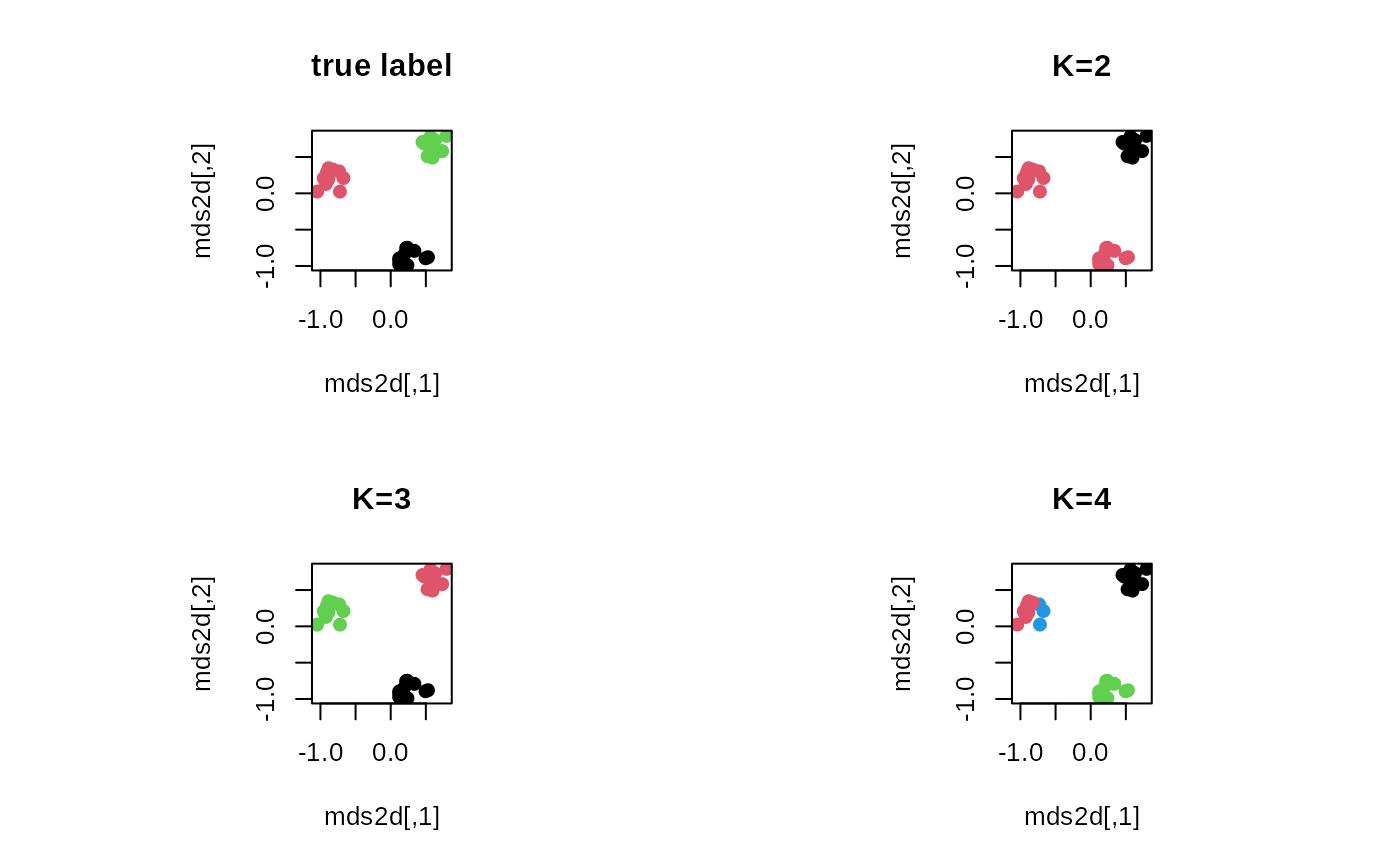
## VISUALIZE
opar <- par(no.readonly=TRUE)
par(mfrow=c(2,2), pty="s")
plot(mds2d, pch=19, main="true label", col=mylabs)
plot(mds2d, pch=19, main="K=2", col=clust2$cluster)
plot(mds2d, pch=19, main="K=3", col=clust3$cluster)
plot(mds2d, pch=19, main="K=4", col=clust4$cluster)
 par(opar)