Given \(N\) observations \(X_1, X_2, \ldots, X_N \in \mathcal{M}\),
perform clustering via Competitive Learning Riemannian Quantization (CLRQ).
Originally, the algorithm is designed for finding voronoi cells that are
used in domain quantization. Given the discrete measure of data, centers of the cells
play a role of cluster centers and data are labeled accordingly based on the distance
to voronoi centers. For an iterative update of centers, gradient descent algorithm
adapted for the Riemannian manifold setting is used with the gain factor sequence
$$\gamma_t = \frac{a}{1 + b \sqrt{t}}$$
where two parameters \(a,b\) are represented by par.a and par.b. For
initialization, we provide k-means++ and random seeding options as in k-means.
Usage
riem.clrq(riemobj, k = 2, init = c("plus", "random"), gain.a = 1, gain.b = 1)Value
a named list containing
- centers
a 3d array where each slice along 3rd dimension is a matrix representation of class centers.
- cluster
a length-\(N\) vector of class labels (from \(1:k\)).
References
Le Brigant A, Puechmorel S (2019). “Quantization and clustering on Riemannian manifolds with an application to air traffic analysis.” Journal of Multivariate Analysis, 173, 685–703. ISSN 0047259X.
Bonnabel S (2013). “Stochastic Gradient Descent on Riemannian Manifolds.” IEEE Transactions on Automatic Control, 58(9), 2217–2229. ISSN 0018-9286, 1558-2523.
Examples
#-------------------------------------------------------------------
#          Example on Sphere : a dataset with three types
#
# class 1 : 10 perturbed data points near (1,0,0) on S^2 in R^3
# class 2 : 10 perturbed data points near (0,1,0) on S^2 in R^3
# class 3 : 10 perturbed data points near (0,0,1) on S^2 in R^3
#-------------------------------------------------------------------
## GENERATE DATA
mydata = list()
for (i in 1:10){
  tgt = c(1, stats::rnorm(2, sd=0.1))
  mydata[[i]] = tgt/sqrt(sum(tgt^2))
}
for (i in 11:20){
  tgt = c(rnorm(1,sd=0.1),1,rnorm(1,sd=0.1))
  mydata[[i]] = tgt/sqrt(sum(tgt^2))
}
for (i in 21:30){
  tgt = c(stats::rnorm(2, sd=0.1), 1)
  mydata[[i]] = tgt/sqrt(sum(tgt^2))
}
myriem = wrap.sphere(mydata)
mylabs = rep(c(1,2,3), each=10)

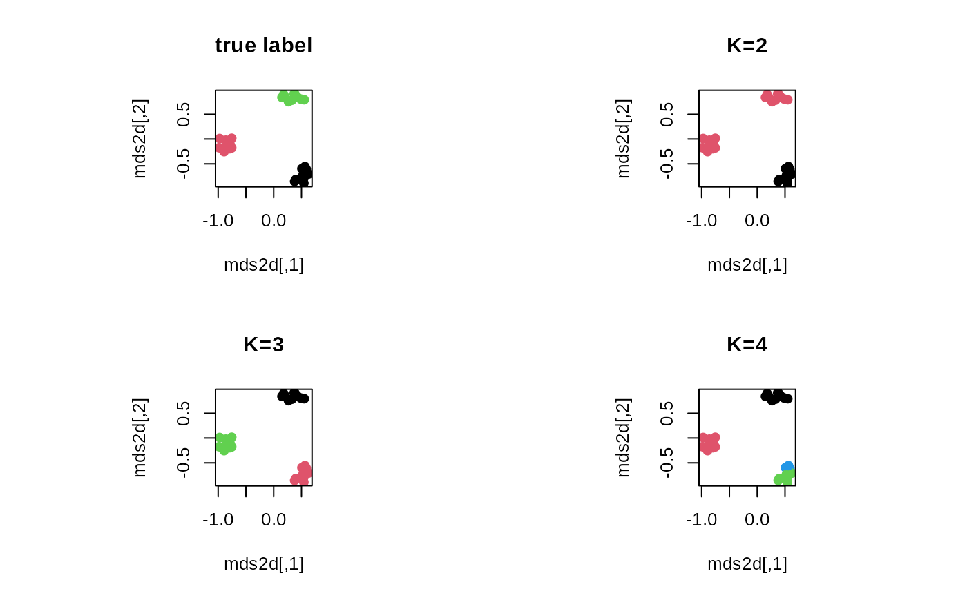
## CLRQ WITH K=2,3,4
clust2 = riem.clrq(myriem, k=2)
clust3 = riem.clrq(myriem, k=3)
clust4 = riem.clrq(myriem, k=4)

## MDS FOR VISUALIZATION
mds2d = riem.mds(myriem, ndim=2)$embed

## VISUALIZE
opar <- par(no.readonly=TRUE)
par(mfrow=c(2,2), pty="s")
plot(mds2d, pch=19, main="true label", col=mylabs)
plot(mds2d, pch=19, main="K=2", col=clust2$cluster)
plot(mds2d, pch=19, main="K=3", col=clust3$cluster)
plot(mds2d, pch=19, main="K=4", col=clust4$cluster)

par(opar)
