Spherical Normal Distribution

We provide tools for an isotropic spherical normal (SN) distributions on a \((p-1)\)-sphere in \(\mathbf{R}^p\) for sampling, density evaluation, and maximum likelihood estimation of the parameters where the density is defined as $$f_{SN}(x; \mu, \lambda) = \frac{1}{Z(\lambda)} \exp \left( -\frac{\lambda}{2} d^2(x,\mu) \right)$$ for location and concentration parameters \(\mu\) and \(\lambda\) respectively and the normalizing constant \(Z(\lambda)\).

Usage

dspnorm(data, mu, lambda, log = FALSE)

rspnorm(n, mu, lambda)

mle.spnorm(data, method = c("Newton", "Halley", "Optimize", "DE"), ...)

Arguments

data

data vectors in form of either an \((n\times p)\) matrix or a length-\(n\) list. See wrap.sphere for descriptions on supported input types.

mu

a length-\(p\) unit-norm vector of location.

lambda

a concentration parameter that is positive.

log

a logical; TRUE to return log-density, FALSE for densities without logarithm applied.

n

the number of samples to be generated.

method

an algorithm name for concentration parameter estimation. It should be one of "Newton","Halley","Optimize", and "DE" (case sensitive).

...

extra parameters for computations, including

maxiter

maximum number of iterations to be run (default:50).

eps

tolerance level for stopping criterion (default: 1e-5).

Value

dspnorm gives a vector of evaluated densities given samples. rspnorm generates unit-norm vectors in \(\mathbf{R}^p\) wrapped in a list. mle.spnorm computes MLEs and returns a list containing estimates of location (mu) and concentration (lambda) parameters.

References

Hauberg S (2018). “Directional Statistics with the Spherical Normal Distribution.” In 2018 21st International Conference on Information Fusion (FUSION), 704–711. ISBN 978-0-9964527-6-2.

You K, Suh C (2022). “Parameter Estimation and Model-Based Clustering with Spherical Normal Distribution on the Unit Hypersphere.” Computational Statistics & Data Analysis, 107457. ISSN 01679473.

Examples

# \donttest{
# -------------------------------------------------------------------
#          Example with Spherical Normal Distribution
#
# Given a fixed set of parameters, generate samples and acquire MLEs.
# Especially, we will see the evolution of estimation accuracy.
# -------------------------------------------------------------------
## DEFAULT PARAMETERS
true.mu  = c(1,0,0,0,0)
true.lbd = 5

## GENERATE DATA N=1000
big.data = rspnorm(1000, true.mu, true.lbd)

## ITERATE FROM 50 TO 1000 by 10
idseq = seq(from=50, to=1000, by=10)
nseq  = length(idseq)

hist.mu  = rep(0, nseq)
hist.lbd = rep(0, nseq)

for (i in 1:nseq){
  small.data = big.data[1:idseq[i]]          # data subsetting
  small.MLE  = mle.spnorm(small.data) # compute MLE
  
  hist.mu[i]  = acos(sum(small.MLE$mu*true.mu)) # difference in mu
  hist.lbd[i] = small.MLE$lambda
}

## VISUALIZE
opar <- par(no.readonly=TRUE)
par(mfrow=c(1,2))
plot(idseq, hist.mu,  "b", pch=19, cex=0.5, main="difference in location")
plot(idseq, hist.lbd, "b", pch=19, cex=0.5, main="concentration param")
abline(h=true.lbd, lwd=2, col="red")

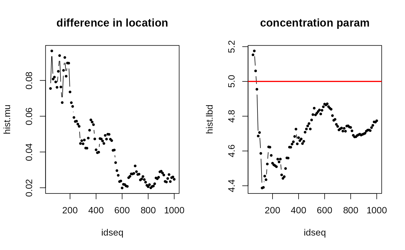par(opar)
# }