Generate Random Samples from Multivariate Normal Distribution

In $\mathbf{R}^p$, random samples are drawn $$X_1,X_2,\ldots,X_n~ \sim ~ \mathcal{N}(\mu, \Sigma)$$ where $\mu \in \mathbf{R}^p$ is a mean vector and $\Sigma \in \textrm{SPD}(p)$ is a positive definite covariance matrix.

Usage

rmvnorm(n = 1, mu, sigma)

Arguments

n: the number of samples to be generated.
mu: mean vector.
sigma: covariance matrix.

Value

either (1) a length-$p$ vector ($n=1$) or (2) an $(n\times p)$ matrix where rows are random samples.

Examples

#-------------------------------------------------------------------
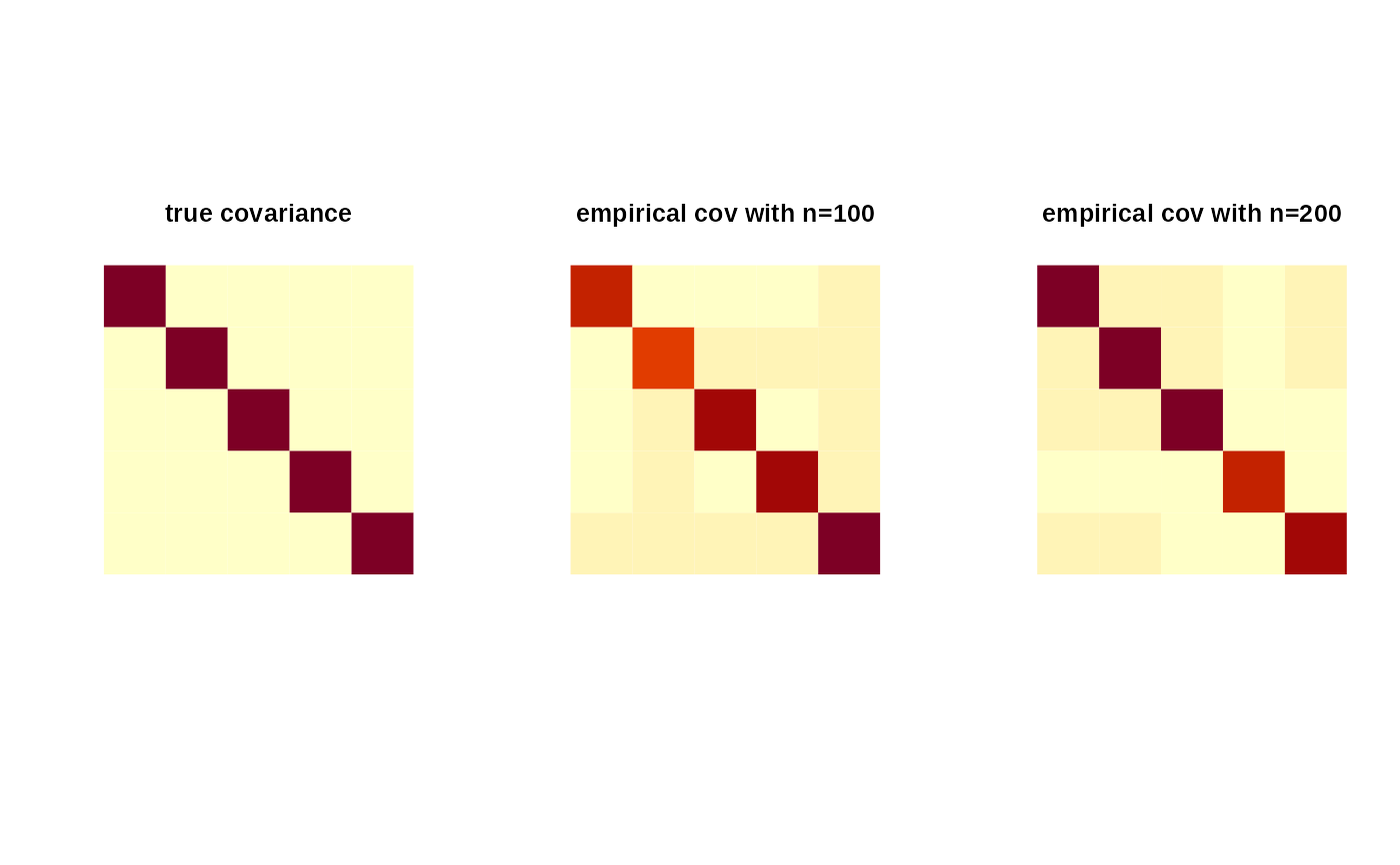
#   Generate Random Data and Compare with Empirical Covariances
#
# In R^5 with zero mean and diagonal covariance, 
# generate 100 and 200 observations and compute MLE covariance.
#-------------------------------------------------------------------
## GENERATE DATA
mymu  = rep(0,5)
mysig = diag(5)

## MLE FOR COVARIANCE
smat1 = stats::cov(rmvnorm(n=100, mymu, mysig))
smat2 = stats::cov(rmvnorm(n=200, mymu, mysig))

## VISUALIZE
opar <- par(no.readonly=TRUE)
par(mfrow=c(1,3), pty="s")
image(mysig[,5:1], axes=FALSE, main="true covariance")
image(smat1[,5:1], axes=FALSE, main="empirical cov with n=100")
image(smat2[,5:1], axes=FALSE, main="empirical cov with n=200")

par(opar)