Given \(N\) observations \(X_1, X_2, \ldots, X_N \in \mathcal{M}\), t-SNE mimicks the pattern of probability distributions over pairs of manifold-valued objects on low-dimensional target embedding space by minimizing Kullback-Leibler divergence.
Usage
riem.tsne(riemobj, ndim = 2, geometry = c("intrinsic", "extrinsic"), ...)Arguments
- riemobj
a S3
"riemdata"class for \(N\) manifold-valued data.- ndim
an integer-valued target dimension.
- geometry
(case-insensitive) name of geometry; either geodesic (
"intrinsic") or embedded ("extrinsic") geometry.- ...
extra parameters for
Rtsnealgorithm from Rtsne package, such as perplexity, momentum, and others.
Value
a named list containing
- embed
an \((N\times ndim)\) matrix whose rows are embedded observations.
- stress
discrepancy between embedded and original distances as a measure of error.
Examples
#-------------------------------------------------------------------
# Example on Sphere : a dataset with three types
#
# 10 perturbed data points near (1,0,0) on S^2 in R^3
# 10 perturbed data points near (0,1,0) on S^2 in R^3
# 10 perturbed data points near (0,0,1) on S^2 in R^3
#-------------------------------------------------------------------
## GENERATE DATA
mydata = list()
for (i in 1:20){
tgt = c(1, stats::rnorm(2, sd=0.1))
mydata[[i]] = tgt/sqrt(sum(tgt^2))
}
for (i in 21:40){
tgt = c(rnorm(1,sd=0.1),1,rnorm(1,sd=0.1))
mydata[[i]] = tgt/sqrt(sum(tgt^2))
}
for (i in 41:60){
tgt = c(stats::rnorm(2, sd=0.1), 1)
mydata[[i]] = tgt/sqrt(sum(tgt^2))
}
myriem = wrap.sphere(mydata)
mylabs = rep(c(1,2,3), each=20)
## RUN THE ALGORITHM IN TWO GEOMETRIES
mypx = 5
embed2int = riem.tsne(myriem, ndim=2, geometry="intrinsic", perplexity=mypx)
embed2ext = riem.tsne(myriem, ndim=2, geometry="extrinsic", perplexity=mypx)
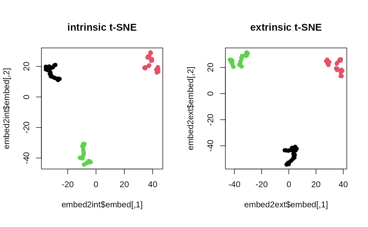
## VISUALIZE
opar = par(no.readonly=TRUE)
par(mfrow=c(1,2), pty="s")
plot(embed2int$embed, main="intrinsic t-SNE", col=mylabs, pch=19)
plot(embed2ext$embed, main="extrinsic t-SNE", col=mylabs, pch=19)
 par(opar)