Given \(N\) observations \(X_1, X_2, \ldots, X_N \in \mathcal{M}\), find the smallest enclosing ball.
Usage
riem.seb(riemobj, method = c("aa2013"), ...)Arguments
- riemobj
a S3
"riemdata"class for \(N\) manifold-valued data.- method
(case-insensitive) name of the algorithm to be used as follows;
"aa2013"Arnaudon and Nielsen (2013).
- ...
extra parameters including
- maxiter
maximum number of iterations to be run (default:50).
- eps
tolerance level for stopping criterion (default: 1e-5).
Value
a named list containing
- center
a matrix on \(\mathcal{M}\) that minimizes the radius.
- radius
the minimal radius with respect to the
center.
References
Bâdoiu M, Clarkson KL (2003). “Smaller core-sets for balls.” In Proceedings of the fourteenth annual ACM-SIAM symposium on discrete algorithms, SODA '03, 801–802. ISBN 0-89871-538-5.
Arnaudon M, Nielsen F (2013). “On approximating the Riemannian 1-center.” Computational Geometry, 46(1), 93–104. ISSN 09257721.
Examples
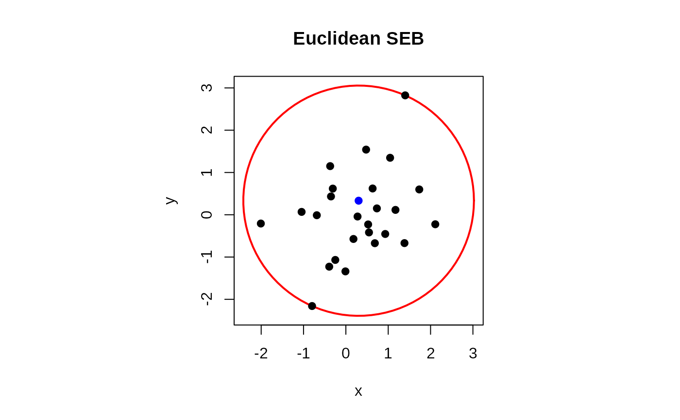
#-------------------------------------------------------------------
#       Euclidean Example : samples from Standard Normal in R^2
#-------------------------------------------------------------------
## GENERATE 25 OBSERVATIONS FROM N(0,I)
ndata  = 25
mymats = array(0,c(ndata, 2))
mydata = list()
for (i in 1:ndata){
  mydata[[i]] = stats::rnorm(2)
  mymats[i,]  = mydata[[i]]
}
myriem = wrap.euclidean(mydata)

## COMPUTE
sebobj = riem.seb(myriem)
center = as.vector(sebobj$center)
radius = sebobj$radius

## VISUALIZE
#  1. prepare the circle for drawing
theta  = seq(from=0, to=2*pi, length.out=100)
coords = radius*cbind(cos(theta), sin(theta))
coords = coords + matrix(rep(center, each=100), ncol=2)

#  2. draw
opar <- par(no.readonly=TRUE)
par(pty="s")
plot(coords, type="l", lwd=2, col="red",
     main="Euclidean SEB", xlab="x", ylab="y")
points(mymats, pch=19)                           # data
points(center[1], center[2], pch=19, col="blue") # center

par(opar)