Spectral Clustering by Ng, Jordan, and Weiss (2002)

The version of Ng, Jordan, and Weiss first constructs the affinity matrix $$A_{ij} = \exp(-d(x_i, d_j)^2 / \sigma^2)$$ where $\sigma$ is a common bandwidth parameter and performs k-means clustering on the row-space of eigenvectors for the symmetric graph laplacian matrix $$L=D^{-1/2}(D-A)D^{-1/2}$$.

Usage

riem.scNJW(riemobj, k = 2, sigma = 1, geometry = c("intrinsic", "extrinsic"))

Arguments

riemobj: a S3 "riemdata" class for $N$ manifold-valued data.
k: the number of clusters (default: 2).
sigma: bandwidth parameter (default: 1).
geometry: (case-insensitive) name of geometry; either geodesic ("intrinsic") or embedded ("extrinsic") geometry.

Value

a named list containing

cluster: a length-$N$ vector of class labels (from $1:k$).
eigval: eigenvalues of the graph laplacian's spectral decomposition.
embeds: an $(N\times k)$ low-dimensional embedding.

References

Ng AY, Jordan MI, Weiss Y (2002). "On Spectral Clustering: Analysis and an Algorithm." In Dietterich TG, Becker S, Ghahramani Z (eds.), Advances in Neural Information Processing Systems 14, 849–856. MIT Press.

Examples

#-------------------------------------------------------------------
#          Example on Sphere : a dataset with three types
#
# class 1 : 10 perturbed data points near (1,0,0) on S^2 in R^3
# class 2 : 10 perturbed data points near (0,1,0) on S^2 in R^3
# class 3 : 10 perturbed data points near (0,0,1) on S^2 in R^3
#-------------------------------------------------------------------
## GENERATE DATA
mydata = list()
for (i in 1:10){
  tgt = c(1, stats::rnorm(2, sd=0.1))
  mydata[[i]] = tgt/sqrt(sum(tgt^2))
}
for (i in 11:20){
  tgt = c(rnorm(1,sd=0.1),1,rnorm(1,sd=0.1))
  mydata[[i]] = tgt/sqrt(sum(tgt^2))
}
for (i in 21:30){
  tgt = c(stats::rnorm(2, sd=0.1), 1)
  mydata[[i]] = tgt/sqrt(sum(tgt^2))
}
myriem = wrap.sphere(mydata)
lab    = rep(c(1,2,3), each=10)

## CLUSTERING WITH DIFFERENT K VALUES
cl2 = riem.scNJW(myriem, k=2)$cluster
cl3 = riem.scNJW(myriem, k=3)$cluster
cl4 = riem.scNJW(myriem, k=4)$cluster

## MDS FOR VISUALIZATION
mds2d = riem.mds(myriem, ndim=2)$embed

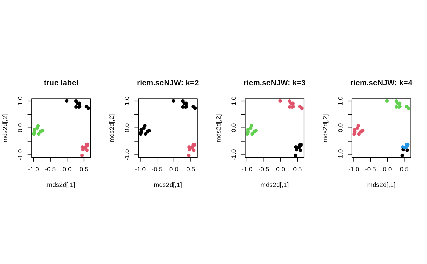
## VISUALIZE
opar <- par(no.readonly=TRUE)
par(mfrow=c(1,4), pty="s")
plot(mds2d, col=lab, pch=19, main="true label")
plot(mds2d, col=cl2, pch=19, main="riem.scNJW: k=2")
plot(mds2d, col=cl3, pch=19, main="riem.scNJW: k=3")
plot(mds2d, col=cl4, pch=19, main="riem.scNJW: k=4")

par(opar)