
Given \(N\) observations \(X_1, X_2, \ldots, X_N \in \mathcal{M}\), apply Sammon mapping, a non-linear dimensionality reduction method. Since the method depends only on the pairwise distances of the data, it can be adapted to the manifold-valued data.
Usage
riem.sammon(riemobj, ndim = 2, geometry = c("intrinsic", "extrinsic"), ...)Arguments
- riemobj
a S3
"riemdata"class for \(N\) manifold-valued data.- ndim
a positive integer target dimension smaller than the number of observations (default: 2).
- geometry
(case-insensitive) name of geometry; either geodesic (
"intrinsic") or embedded ("extrinsic") geometry.- ...
named controls including
- maxiter
positive maximum number of iterations (default: 50).
- eps
nonnegative tolerance for the root mean squared coordinate step, after distances are divided by their maximum (default: 1e-5).
Unknown controls are errors.
Value
a named list containing
- embed
an \((N\times ndim)\) matrix whose rows are embedded observations.
- stress
normalized distance stress, \(\sqrt{\sum_{i<j}(D_{ij}-d_{ij})^2/\sum_{i<j}D_{ij}^2}\). This legacy diagnostic differs from the optimized Sammon loss.
Details
The optimized Sammon loss is \(\sum_{i<j}(D_{ij}-d_{ij})^2/D_{ij}\,/\,\sum_{i<j}D_{ij}\), where \(D\) and \(d\) are the original and embedded distances. Every off-diagonal original distance must be strictly positive and finite; coincident observations (including different representations of the same point) must be removed before fitting because this loss divides by \(D_{ij}\). Distances are normalized internally, making the stopping tolerance independent of a common change of measurement units. Classical scaling initializes the coordinates, with negative eigenvalues truncated to zero and coincident projected points separated by a small deterministic perturbation. Diagonal-Hessian updates use backtracking to decrease the Sammon loss. If no finite decreasing step can be found, the last accepted coordinates are returned. This local procedure does not establish a global minimum.
Validation status
This retained legacy interface is experimental. Its full numerical and
statistical contract has not been independently verified across supported
inputs. See riem-method-contracts and the installed contract
table for method-specific assumptions, restrictions, and evidence scope.
References
Sammon JW (1969). “A Nonlinear Mapping for Data Structure Analysis.” IEEE Transactions on Computers, C-18(5), 401–409. ISSN 0018-9340.
Examples
#-------------------------------------------------------------------
# Example on Sphere : a dataset with three types
#
# 10 perturbed data points near (1,0,0) on S^2 in R^3
# 10 perturbed data points near (0,1,0) on S^2 in R^3
# 10 perturbed data points near (0,0,1) on S^2 in R^3
#-------------------------------------------------------------------
## GENERATE DATA
mydata = list()
for (i in 1:10){
tgt = c(1, stats::rnorm(2, sd=0.1))
mydata[[i]] = tgt/sqrt(sum(tgt^2))
}
for (i in 11:20){
tgt = c(rnorm(1,sd=0.1),1,rnorm(1,sd=0.1))
mydata[[i]] = tgt/sqrt(sum(tgt^2))
}
for (i in 21:30){
tgt = c(stats::rnorm(2, sd=0.1), 1)
mydata[[i]] = tgt/sqrt(sum(tgt^2))
}
myriem = wrap.sphere(mydata)
mylabs = rep(c(1,2,3), each=10)
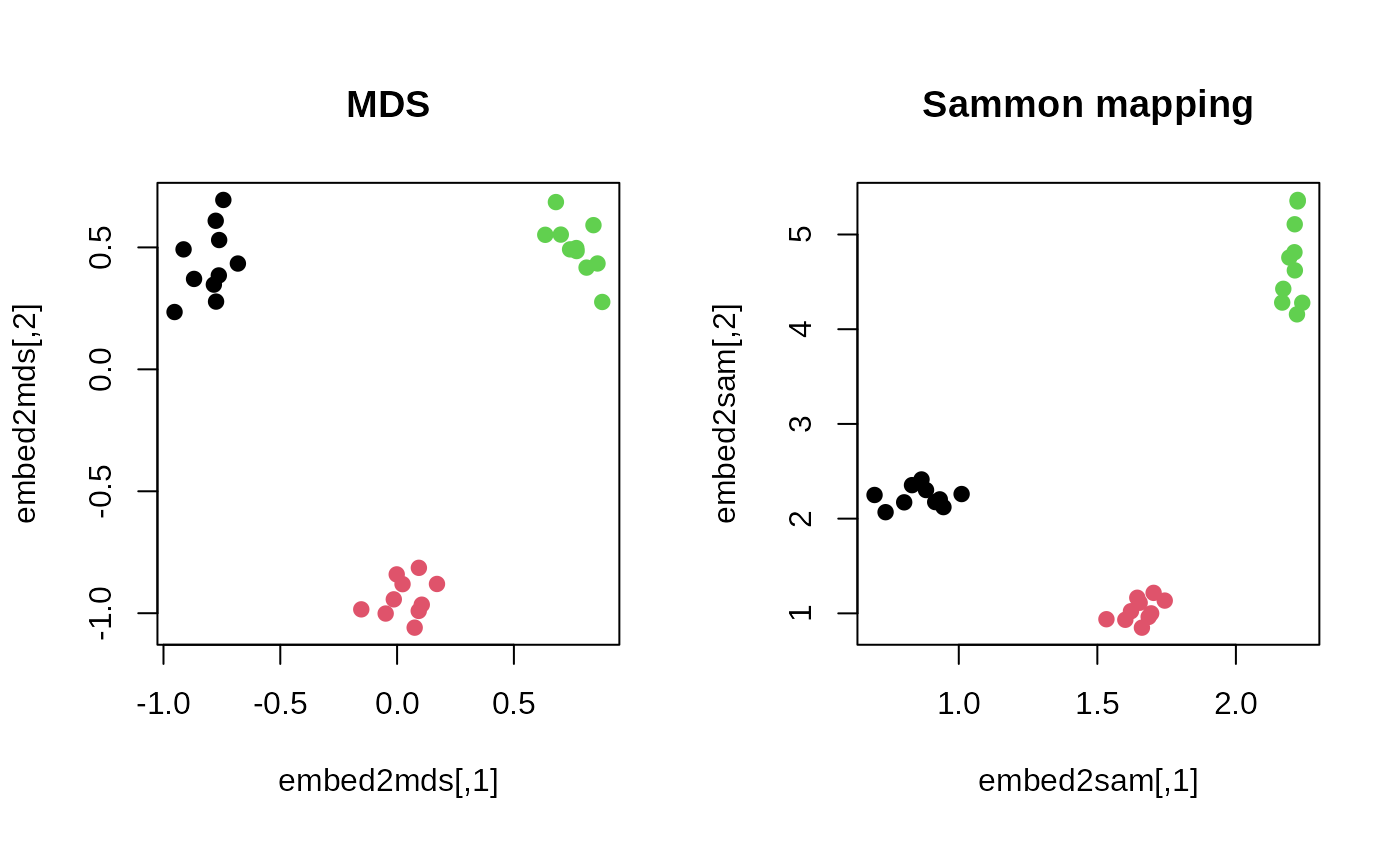
## COMPARE SAMMON WITH MDS
embed2mds = riem.mds(myriem, ndim=2)$embed
embed2sam = riem.sammon(myriem, ndim=2)$embed
## VISUALIZE
opar = par(no.readonly=TRUE)
par(mfrow=c(1,2), pty="s")
plot(embed2mds, col=mylabs, pch=19, main="MDS")
plot(embed2sam, col=mylabs, pch=19, main="Sammon mapping")
 par(opar)