Manifold-to-Scalar Kernel Regression with K-Fold Cross Validation

Usage

riem.m2skregCV(
  riemobj,
  y,
  bandwidths = seq(from = 0.01, to = 1, length.out = 10),
  geometry = c("intrinsic", "extrinsic"),
  kfold = 5
)

Arguments

riemobj: a S3 "riemdata" class for \(N\) manifold-valued data corresponding to \(X_1,\ldots,X_N\).
y: a length-\(N\) vector of dependent variable values.
bandwidths: a vector of nonnegative numbers that control smoothness.
geometry: (case-insensitive) name of geometry; either geodesic ("intrinsic") or embedded ("extrinsic") geometry.
kfold: the number of folds for cross validation.

Value

a named list of S3 class m2skreg containing

ypred: a length-\(N\) vector of optimal smoothed responses.
bandwidth: the optimal bandwidth value.
inputs: a list containing both riemobj and y for future use.
errors: a matrix whose columns are bandwidths values and corresponding errors measure in SSE.

Examples

# \donttest{
#-------------------------------------------------------------------
#                    Example on Sphere S^2
#
#  X : equi-spaced points from (0,0,1) to (0,1,0)
#  y : sin(x) with perturbation
#-------------------------------------------------------------------
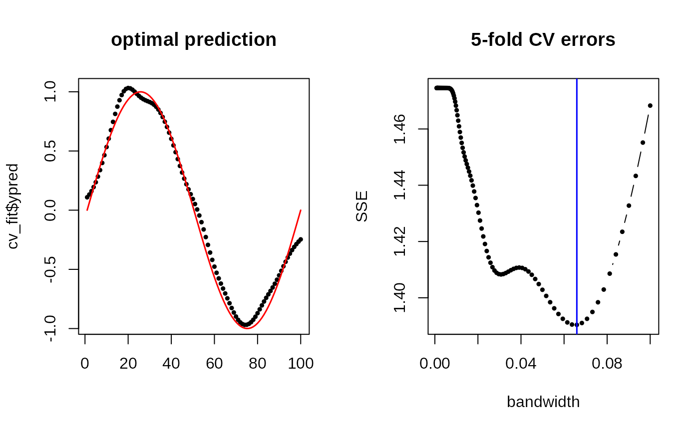
# GENERATE DATA
set.seed(496) 
npts = 100
nlev = 0.25
thetas = seq(from=0, to=pi/2, length.out=npts)
Xstack = cbind(rep(0,npts), sin(thetas), cos(thetas))

Xriem  = wrap.sphere(Xstack)
ytrue  = sin(seq(from=0, to=2*pi, length.out=npts))
ynoise = ytrue + rnorm(npts, sd=nlev)

# FIT WITH 5-FOLD CV
cv_band = (10^seq(from=-4, to=-1, length.out=200))
cv_fit  = riem.m2skregCV(Xriem, ynoise, bandwidths=cv_band)
cv_err  = cv_fit$errors

# VISUALIZE
opar <- par(no.readonly=TRUE)
par(mfrow=c(1,2))
plot(1:npts, cv_fit$ypred, pch=19, cex=0.5, "b", xlab="", main="optimal prediction")
lines(1:npts, ytrue, col="red", lwd=1.5)
plot(cv_err[,1], cv_err[,2], "b", pch=19, cex=0.5, main="5-fold CV errors",
     xlab="bandwidth", ylab="SSE")
abline(v=cv_fit$bandwidth, col="blue", lwd=1.5)

par(opar)
# }