Although the method of Kernel Principal Component Analysis (KPCA) was originally developed to visualize non-linearly distributed data in Euclidean space, we graft this to the case for manifolds where extrinsic geometry is explicitly available. The algorithm uses Gaussian kernel with $$K(X_i, X_j) = \exp\left( - \frac{d^2 (X_i, X_j)}{2 \sigma^2} \right )$$ where \(\sigma\) is a bandwidth parameter and \(d(\cdot, \cdot)\) is an extrinsic distance defined on a specific manifold.
Value
a named list containing
- embed
an \((N\times ndim)\) matrix whose rows are embedded observations.
- vars
a length-\(N\) vector of eigenvalues from kernelized covariance matrix.
References
Schölkopf B, Smola A, Müller K (1997). “Kernel principal component analysis.” In Goos G, Hartmanis J, van Leeuwen J, Gerstner W, Germond A, Hasler M, Nicoud J (eds.), Artificial Neural Networks — ICANN'97, volume 1327, 583–588. Springer Berlin Heidelberg, Berlin, Heidelberg. ISBN 978-3-540-63631-1 978-3-540-69620-9.
Examples
#-------------------------------------------------------------------
# Example for Gorilla Skull Data : 'gorilla'
#-------------------------------------------------------------------
## PREPARE THE DATA
# Aggregate two classes into one set
data(gorilla)
mygorilla = array(0,c(8,2,59))
for (i in 1:29){
mygorilla[,,i] = gorilla$male[,,i]
}
for (i in 30:59){
mygorilla[,,i] = gorilla$female[,,i-29]
}
gor.riem = wrap.landmark(mygorilla)
gor.labs = c(rep("red",29), rep("blue",30))
## APPLY KPCA WITH DIFFERENT KERNEL BANDWIDTHS
kpca1 = riem.kpca(gor.riem, sigma=0.01)
kpca2 = riem.kpca(gor.riem, sigma=1)
kpca3 = riem.kpca(gor.riem, sigma=100)
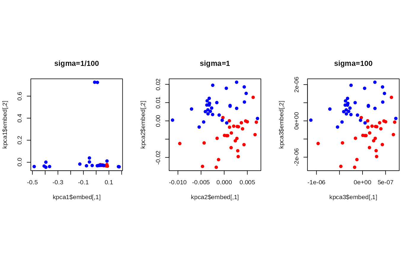
## VISUALIZE
opar <- par(no.readonly=TRUE)
par(mfrow=c(1,3), pty="s")
plot(kpca1$embed, pch=19, col=gor.labs, main="sigma=1/100")
plot(kpca2$embed, pch=19, col=gor.labs, main="sigma=1")
plot(kpca3$embed, pch=19, col=gor.labs, main="sigma=100")
 par(opar)