Isometric Feature Mapping

ISOMAP - isometric feature mapping - is a dimensionality reduction method to apply classical multidimensional scaling to the geodesic distance that is computed on a weighted nearest neighborhood graph. Nearest neighbor is defined by \(k\)-NN where two observations are said to be connected when they are mutually included in each other's nearest neighbor. Note that it is possible for geodesic distances to be Inf when nearest neighbor graph construction incurs separate connected components. When an extra parameter padding=TRUE, infinite distances are replaced by 2 times the maximal finite geodesic distance.

Usage

riem.isomap(
  riemobj,
  ndim = 2,
  nnbd = 5,
  geometry = c("intrinsic", "extrinsic"),
  ...
)

Arguments

riemobj

a S3 "riemdata" class for \(N\) manifold-valued data.

ndim

an integer-valued target dimension (default: 2).

nnbd

the size of nearest neighborhood (default: 5).

geometry

(case-insensitive) name of geometry; either geodesic ("intrinsic") or embedded ("extrinsic") geometry.

...

extra parameters including

padding

a logical; if TRUE, Inf-valued geodesic distances are replaced by 2 times the maximal geodesic distance in the data.

Value

a named list containing

embed

an \((N\times ndim)\) matrix whose rows are embedded observations.

References

Silva VD, Tenenbaum JB (2003). “Global Versus Local Methods in Nonlinear Dimensionality Reduction.” In Becker S, Thrun S, Obermayer K (eds.), Advances in Neural Information Processing Systems 15, 721--728. MIT Press.

Examples

#-------------------------------------------------------------------
#          Example on Sphere : a dataset with three types
#
# 10 perturbed data points near (1,0,0) on S^2 in R^3
# 10 perturbed data points near (0,1,0) on S^2 in R^3
# 10 perturbed data points near (0,0,1) on S^2 in R^3
#-------------------------------------------------------------------
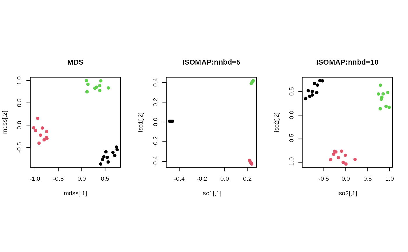
## GENERATE DATA
mydata = list()
for (i in 1:10){
  tgt = c(1, stats::rnorm(2, sd=0.1))
  mydata[[i]] = tgt/sqrt(sum(tgt^2))
}
for (i in 11:20){
  tgt = c(rnorm(1,sd=0.1),1,rnorm(1,sd=0.1))
  mydata[[i]] = tgt/sqrt(sum(tgt^2))
}
for (i in 21:30){
  tgt = c(stats::rnorm(2, sd=0.1), 1)
  mydata[[i]] = tgt/sqrt(sum(tgt^2))
}
myriem = wrap.sphere(mydata)
mylabs = rep(c(1,2,3), each=10)

## MDS AND ISOMAP WITH DIFFERENT NEIGHBORHOOD SIZE
mdss = riem.mds(myriem)$embed
iso1 = riem.isomap(myriem, nnbd=5)$embed
#> [1] "* riem.isomap : some of the geodesic distances are Inf, so 'padding' is applied."
iso2 = riem.isomap(myriem, nnbd=10)$embed

## VISUALIZE
opar = par(no.readonly=TRUE)
par(mfrow=c(1,3), pty="s")
plot(mdss, col=mylabs, pch=19, main="MDS")
plot(iso1, col=mylabs, pch=19, main="ISOMAP:nnbd=5")
plot(iso2, col=mylabs, pch=19, main="ISOMAP:nnbd=10")

par(opar)