Prediction for Manifold-to-Scalar Kernel Regression

Given new observations \(X_1, X_2, \ldots, X_M \in \mathcal{M}\), plug in the data with respect to the fitted model for prediction.

Usage

# S3 method for m2skreg
predict(object, newdata, geometry = c("intrinsic", "extrinsic"), ...)

Arguments

object

an object of m2skreg class. See riem.m2skreg for more details.

newdata

a S3 "riemdata" class for manifold-valued data corresponding to \(X_1,\ldots,X_M\).

geometry

(case-insensitive) name of geometry; either geodesic ("intrinsic") or embedded ("extrinsic") geometry.

...

further arguments passed to or from other methods.

Value

a length-\(M\) vector of predictted values.

See also

riem.m2skreg

Examples

# \donttest{
#-------------------------------------------------------------------
#                    Example on Sphere S^2
#
#  X : equi-spaced points from (0,0,1) to (0,1,0)
#  y : sin(x) with perturbation
#
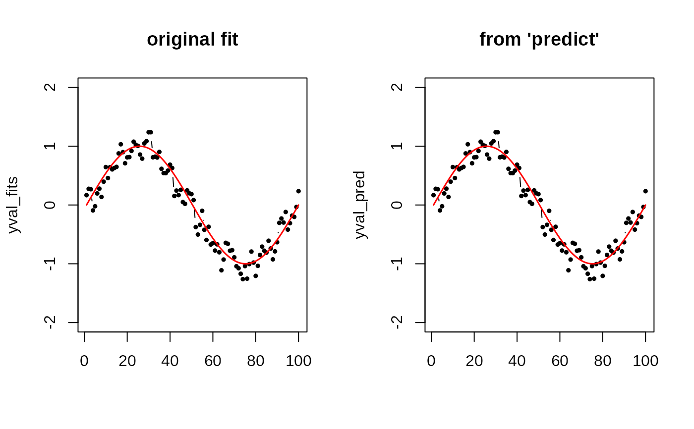
#  Our goal is to check whether the predict function works well
#  by comparing the originally predicted values vs. those of the same data.
#-------------------------------------------------------------------
# GENERATE DATA
npts = 100
nlev = 0.25
thetas = seq(from=0, to=pi/2, length.out=npts)
Xstack = cbind(rep(0,npts), sin(thetas), cos(thetas))

Xriem  = wrap.sphere(Xstack)
ytrue  = sin(seq(from=0, to=2*pi, length.out=npts))
ynoise = ytrue + rnorm(npts, sd=nlev)

# FIT & PREDICT
obj_fit   = riem.m2skreg(Xriem, ynoise, bandwidth=0.01)
yval_fits = obj_fit$ypred
yval_pred = predict(obj_fit, Xriem)

# VISUALIZE
xgrd <- 1:npts
opar <- par(no.readonly=TRUE)
par(mfrow=c(1,2))
plot(xgrd, yval_fits, pch=19, cex=0.5, "b", xlab="", ylim=c(-2,2), main="original fit")
lines(xgrd, ytrue, col="red", lwd=1.5)
plot(xgrd, yval_pred, pch=19, cex=0.5, "b", xlab="", ylim=c(-2,2), main="from 'predict'")
lines(xgrd, ytrue, col="red", lwd=1.5)

par(opar)
# }