Finite Mixture of Spherical Normal Distributions

For $n$ observations on a $(p-1)$ sphere in $\mathbf{R}^p$, a finite mixture model is fitted whose components are spherical normal distributions via the following model $$f(x; \left\lbrace w_k, \mu_k, \lambda_k \right\rbrace_{k=1}^K) = \sum_{k=1}^K w_k SN(x; \mu_k, \lambda_k)$$ with parameters $w_k$'s for component weights, $\mu_k$'s for component locations, and $\lambda_k$'s for component concentrations.

Usage

moSN(
  data,
  k = 2,
  same.lambda = FALSE,
  variants = c("soft", "hard", "stochastic"),
  ...
)

# S3 method for moSN
loglkd(object, newdata)

# S3 method for moSN
label(object, newdata)

# S3 method for moSN
density(object, newdata)

Arguments

data

data vectors in form of either an $(n\times p)$ matrix or a length-$n$ list. See wrap.sphere for descriptions on supported input types.

k

the number of clusters (default: 2).

same.lambda

a logical; TRUE to use same concentration parameter across all components, or FALSE otherwise.

variants

type of the class assignment methods, one of "soft","hard", and "stochastic".

...

extra parameters including

maxiter: the maximum number of iterations (default: 50).
eps: stopping criterion for the EM algorithm (default: 1e-6).
printer: a logical; TRUE to show history of the algorithm, FALSE otherwise.

object

a fitted moSN model from the moSN function.

newdata

data vectors in form of either an $(m\times p)$ matrix or a length-$m$ list. See wrap.sphere for descriptions on supported input types.

Value

a named list of S3 class riemmix containing

cluster: a length-$n$ vector of class labels (from $1:k$).
loglkd: log likelihood of the fitted model.
criteria: a vector of information criteria.
parameters: a list containing proportion, center, and concentration. See the section for more details.
membership: an $(n\times k)$ row-stochastic matrix of membership.

Parameters of the fitted model

A fitted model is characterized by three parameters. For $k$-mixture model on a $(p-1)$ sphere in $\mathbf{R}^p$, (1) proportion is a length-$k$ vector of component weight that sums to 1, (2) center is an $(k\times p)$ matrix whose rows are cluster centers, and (3) concentration is a length-$k$ vector of concentration parameters for each component.

Note on S3 methods

There are three S3 methods; loglkd, label, and density. Given a random sample of size $m$ as newdata, (1) loglkd returns a scalar value of the computed log-likelihood, (2) label returns a length-$m$ vector of cluster assignments, and (3) density evaluates densities of every observation according ot the model fit.

References

You K, Suh C (2022). “Parameter Estimation and Model-Based Clustering with Spherical Normal Distribution on the Unit Hypersphere.” Computational Statistics \& Data Analysis, 107457. ISSN 01679473.

Examples

# \donttest{
# ---------------------------------------------------- #
#                 FITTING THE MODEL
# ---------------------------------------------------- #
# Load the 'city' data and wrap as 'riemobj'
data(cities)
locations = cities$cartesian
embed2    = array(0,c(60,2)) 
for (i in 1:60){
   embed2[i,] = sphere.xyz2geo(locations[i,])
}

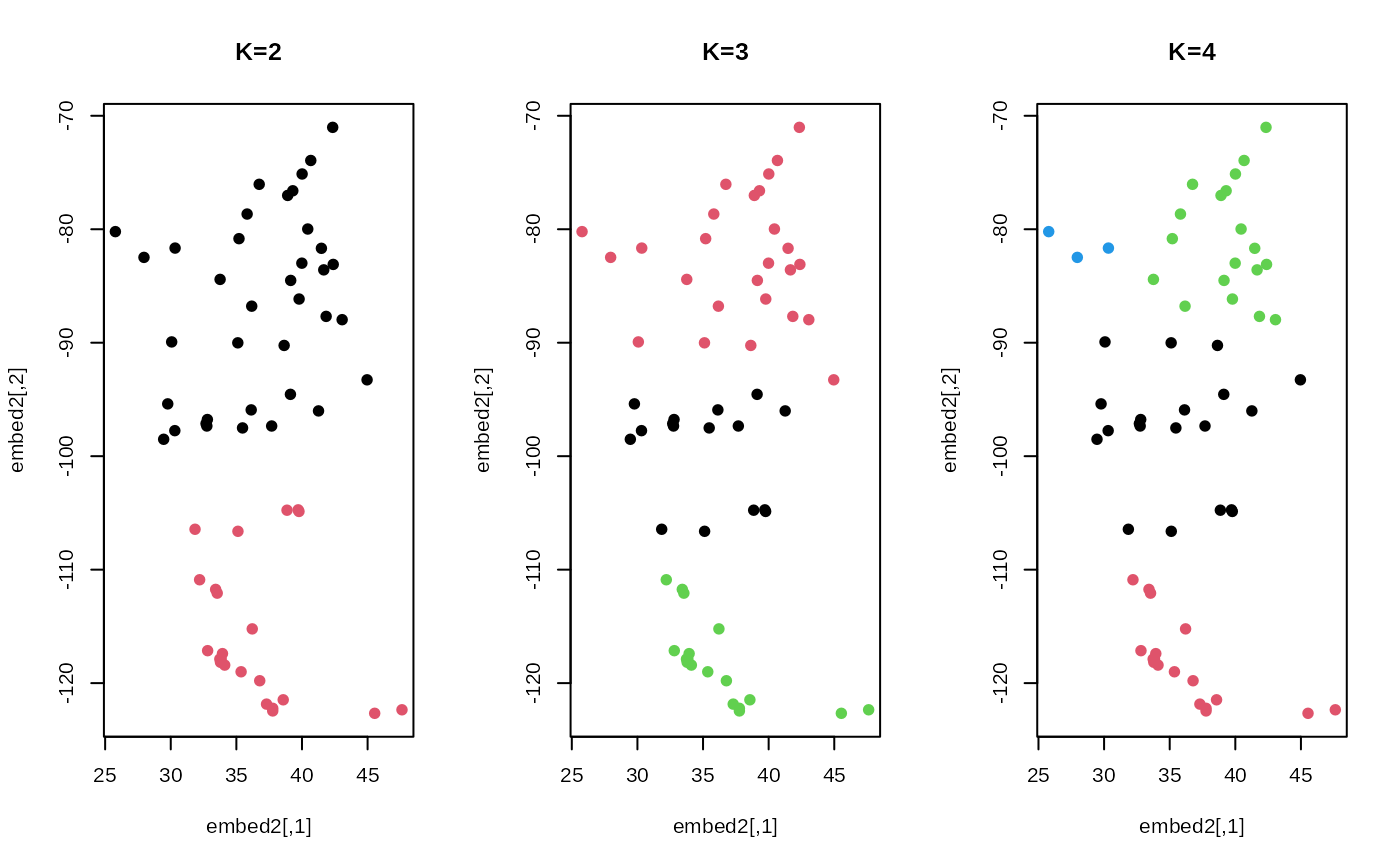
# Fit the model with different numbers of clusters
k2 = moSN(locations, k=2)
k3 = moSN(locations, k=3)
k4 = moSN(locations, k=4)

# Visualize
opar <- par(no.readonly=TRUE)
par(mfrow=c(1,3))
plot(embed2, col=k2$cluster, pch=19, main="K=2")
plot(embed2, col=k3$cluster, pch=19, main="K=3")
plot(embed2, col=k4$cluster, pch=19, main="K=4")

par(opar)

# ---------------------------------------------------- #
#                   USE S3 METHODS
# ---------------------------------------------------- #
# Use the same 'locations' data as new data 
# (1) log-likelihood
newloglkd = round(loglkd(k3, locations), 3)
print(paste0("Log-likelihood for K=3 model fit : ", newloglkd))
#> [1] "Log-likelihood for K=3 model fit : 88.582"

# (2) label
newlabel = label(k3, locations)

# (3) density
newdensity = density(k3, locations)
# }