Angular Central Gaussian Distribution

For a hypersphere $\mathcal{S}^{p-1}$ in $\mathbf{R}^p$, Angular Central Gaussian (ACG) distribution $ACG_p (A)$ is defined via a density $$f(x\vert A) = |A|^{-1/2} (x^\top A^{-1} x)^{-p/2}$$ with respect to the uniform measure on $\mathcal{S}^{p-1}$ and $A$ is a symmetric positive-definite matrix. Since $f(x\vert A) = f(-x\vert A)$, it can also be used as an axial distribution on real projective space, which is unit sphere modulo $\lbrace{+1,-1\rbrace}$. One constraint we follow is that $f(x\vert A) = f(x\vert cA)$ for $c > 0$ in that we use a normalized version for numerical stability by restricting $tr(A)=p$.

Usage

dacg(datalist, A)

racg(n, A)

mle.acg(datalist, ...)

Arguments

datalist

a list of length-$p$ unit-norm vectors.

A

a $(p\times p)$ symmetric positive-definite matrix.

n

the number of samples to be generated.

...

extra parameters for computations, including

maxiter: maximum number of iterations to be run (default:50).
eps: tolerance level for stopping criterion (default: 1e-5).

Value

dacg gives a vector of evaluated densities given samples. racg generates unit-norm vectors in $\mathbf{R}^p$ wrapped in a list. mle.acg estimates the SPD matrix $A$.

References

Tyler DE (1987). “Statistical analysis for the angular central Gaussian distribution on the sphere.” Biometrika, 74(3), 579--589. ISSN 0006-3444, 1464-3510.

Mardia KV, Jupp PE (eds.) (1999). Directional Statistics, Wiley Series in Probability and Statistics. John Wiley \& Sons, Inc., Hoboken, NJ, USA. ISBN 978-0-470-31697-9 978-0-471-95333-3.

Examples

# -------------------------------------------------------------------
#          Example with Angular Central Gaussian Distribution
#
# Given a fixed A, generate samples and estimate A via ML.
# -------------------------------------------------------------------
## GENERATE AND MLE in R^5
#  Generate data
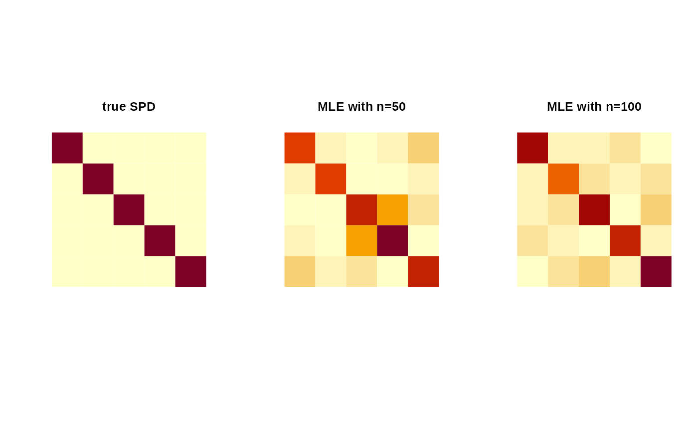
Atrue = diag(5)          # true SPD matrix
sam1  = racg(50,  Atrue) # random samples
sam2  = racg(100, Atrue)

#  MLE
Amle1 = mle.acg(sam1)
Amle2 = mle.acg(sam2)

#  Visualize
opar <- par(no.readonly=TRUE)
par(mfrow=c(1,3), pty="s")
image(Atrue[,5:1], axes=FALSE, main="true SPD")
image(Amle1[,5:1], axes=FALSE, main="MLE with n=50")
image(Amle2[,5:1], axes=FALSE, main="MLE with n=100")

par(opar)