Curvilinear Distance Analysis (CRDA) is a variant of Curvilinear Component Analysis in that the input pairwise distance is altered by curvilinear distance on a data manifold. Like in Isomap, it first generates neighborhood graph and finds shortest path on a constructed graph so that the shortest-path length plays as an approximate geodesic distance on nonlinear manifolds.
do.crda(
  X,
  ndim = 2,
  type = c("proportion", 0.1),
  symmetric = "union",
  weight = TRUE,
  lambda = 1,
  alpha = 1,
  maxiter = 1000,
  tolerance = 1e-06
)
Arguments
- X
an \((n\times p)\) matrix or data frame whose rows are observations and columns represent independent variables.
- ndim
an integer-valued target dimension.
- type
a vector of neighborhood graph construction. Following types are supported;
c("knn",k),c("enn",radius), andc("proportion",ratio). Default isc("proportion",0.1), connecting about 1/10 of nearest data points among all data points. See alsoaux.graphnbdfor more details.- symmetric
one of
"intersect","union"or"asymmetric"is supported. Default is"union". See alsoaux.graphnbdfor more details.- weight
TRUEto perform CRDA on weighted graph, orFALSEotherwise.- lambda
threshold value.
- alpha
initial value for updating.
- maxiter
maximum number of iterations allowed.
- tolerance
stopping criterion for maximum absolute discrepancy between two distance matrices.
Value
a named list containing
- Y
an \((n\times ndim)\) matrix whose rows are embedded observations.
- niter
the number of iterations until convergence.
- trfinfo
a list containing information for out-of-sample prediction.
References
Lee JA, Lendasse A, Verleysen M (2002). “Curvilinear Distance Analysis versus Isomap.” In ESANN.
Lee JA, Lendasse A, Verleysen M (2004). “Nonlinear Projection with Curvilinear Distances: Isomap versus Curvilinear Distance Analysis.” Neurocomputing, 57, 49--76.
Examples
## load iris data
data(iris)
set.seed(100)
subid = sample(1:150,50)
X = as.matrix(iris[subid,1:4])
label = as.factor(iris[subid,5])
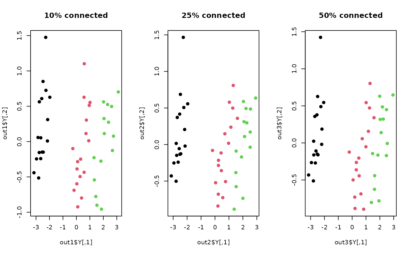
## different settings of connectivity
out1 <- do.crda(X, type=c("proportion",0.10))
out2 <- do.crda(X, type=c("proportion",0.25))
out3 <- do.crda(X, type=c("proportion",0.50))
## visualize
opar <- par(no.readonly=TRUE)
par(mfrow=c(1,3))
plot(out1$Y, col=label, pch=19, main="10% connected")
plot(out2$Y, col=label, pch=19, main="25% connected")
plot(out3$Y, col=label, pch=19, main="50% connected")
 par(opar)