Curvilinear Component Analysis

Curvilinear Component Analysis (CRCA) is a type of self-organizing algorithms for manifold learning. Like MDS, it aims at minimizing a cost function (Stress) based on pairwise proximity. Parameter lambda is a heaviside function for penalizing distance pair of embedded data, and alpha controls learning rate similar to that of subgradient method in that at each iteration \(t\) the gradient is weighted by \(\alpha /t\).

do.crca(X, ndim = 2, lambda = 1, alpha = 1, maxiter = 1000, tolerance = 1e-06)

Arguments

X

an \((n\times p)\) matrix or data frame whose rows are observations and columns represent independent variables.

ndim

an integer-valued target dimension.

lambda

threshold value.

alpha

initial value for updating.

maxiter

maximum number of iterations allowed.

tolerance

stopping criterion for maximum absolute discrepancy between two distance matrices.

Value

a named list containing

Y

an \((n\times ndim)\) matrix whose rows are embedded observations.

niter

the number of iterations until convergence.

trfinfo

a list containing information for out-of-sample prediction.

References

Demartines P, Herault J (1997). “Curvilinear Component Analysis: A Self-Organizing Neural Network for Nonlinear Mapping of Data Sets.” IEEE Transactions on Neural Networks, 8(1), 148--154.

Hérault J, Jausions-Picaud C, Guérin-Dugué A (1999). “Curvilinear Component Analysis for High-Dimensional Data Representation: I. Theoretical Aspects and Practical Use in the Presence of Noise.” In Goos G, Hartmanis J, van Leeuwen J, Mira J, Sánchez-Andrés JV (eds.), Engineering Applications of Bio-Inspired Artificial Neural Networks, volume 1607, 625--634. Springer Berlin Heidelberg, Berlin, Heidelberg. ISBN 978-3-540-66068-2 978-3-540-48772-2.

See also

do.crda

Author

Kisung You

Examples

## use iris data
data(iris)
set.seed(100)
subid = sample(1:150, 50)
X     = as.matrix(iris[subid,1:4])
label = as.factor(iris[subid,5])

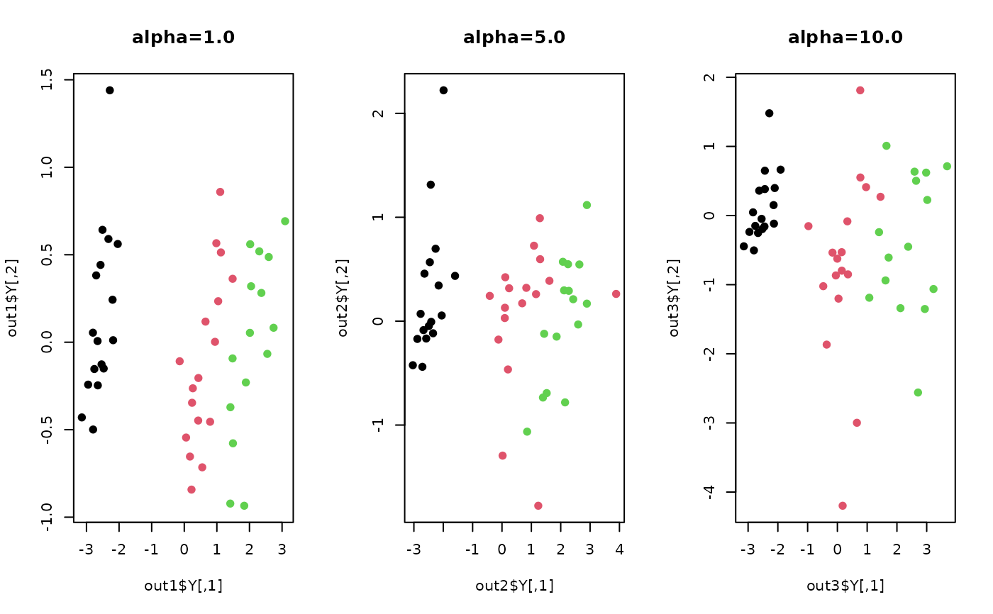
## different initial learning rates
out1 <- do.crca(X,alpha=1)
out2 <- do.crca(X,alpha=5)
out3 <- do.crca(X,alpha=10)

## visualize
opar <- par(no.readonly=TRUE)
par(mfrow=c(1,3))
plot(out1$Y, col=label, pch=19, main="alpha=1.0")
plot(out2$Y, col=label, pch=19, main="alpha=5.0")
plot(out3$Y, col=label, pch=19, main="alpha=10.0")

par(opar)