Construct Nearest-Neighborhood Graph

Given data, it first computes pairwise distance (method) using one of measures defined from dist function. Then, type controls how nearest neighborhood graph should be constructed. Finally, symmetric parameter controls how nearest neighborhood graph should be symmetrized.

aux.graphnbd(
  data,
  method = "euclidean",
  type = c("proportion", 0.1),
  symmetric = "union",
  pval = 2
)

Arguments

data

an \((n\times p)\) data matrix.

method

type of distance to be used. See also dist.

type

a defining pattern of neighborhood criterion. One of

c("knn", k)

knn with k a positive integer.

c("enn", radius)

enn with a positive radius.

c("proportion", ratio)

takes an ratio in (0,1) portion of edges to be connected.

symmetric

either ``intersect'' or ``union'' for symmetrization, or ``asymmetric''.

pval

a \(p\)-norm option for Minkowski distance.

Value

a named list containing

mask

a binary matrix of indicating existence of an edge for each element.

dist

corresponding distance matrix. -Inf is returned for non-connecting edges.

Nearest Neighbor(NN) search

Our package supports three ways of defining nearest neighborhood. First is knn, which finds k nearest points and flag them as neighbors. Second is enn - epsilon nearest neighbor - that connects all the data poinst within a certain radius. Finally, proportion flag is to connect proportion-amount of data points sequentially from the nearest to farthest.

Symmetrization

In many graph setting, it starts from dealing with undirected graphs. NN search, however, does not necessarily guarantee if symmetric connectivity would appear or not. There are two easy options for symmetrization; intersect for connecting two nodes if both of them are nearest neighbors of each other and union for only either of them to be present.

Author

Kisung You

Examples

# \donttest{
## Generate data
set.seed(100)
X = aux.gensamples(n=100)

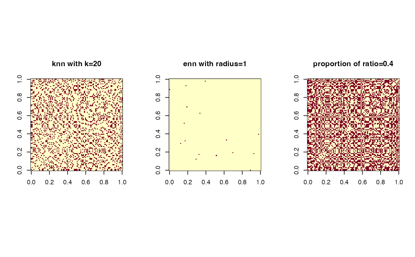
## Test three different types of neighborhood connectivity
nn1 = aux.graphnbd(X,type=c("knn",20))         # knn with k=20
nn2 = aux.graphnbd(X,type=c("enn",1))          # enn with radius = 1
nn3 = aux.graphnbd(X,type=c("proportion",0.4)) # connecting 40% of edges

## Visualize
opar <- par(no.readonly=TRUE)
par(mfrow=c(1,3), pty="s")
image(nn1$mask); title("knn with k=20")
image(nn2$mask); title("enn with radius=1")
image(nn3$mask); title("proportion of ratio=0.4")

par(opar)
# }