Kernel-Weighted Unsupervised Discriminant Projection

Kernel-Weighted Unsupervised Discriminant Projection (KUDP) is a generalization of UDP where proximity is given by weighted values via heat kernel, $$K_{i,j} = \exp(-\|x_i-x_j\|^2/bandwidth)$$ whence UDP uses binary connectivity. If bandwidth is $+\infty$, it becomes a standard UDP problem. Like UDP, it also performs PCA preprocessing for rank-deficient case.

do.kudp(
  X,
  ndim = 2,
  type = c("proportion", 0.1),
  preprocess = c("center", "scale", "cscale", "decorrelate", "whiten"),
  bandwidth = 1
)

Arguments

X: an $(n\times p)$ matrix or data frame whose rows are observations and columns represent independent variables.
ndim: an integer-valued target dimension.
type: a vector of neighborhood graph construction. Following types are supported; c("knn",k), c("enn",radius), and c("proportion",ratio). Default is c("proportion",0.1), connecting about 1/10 of nearest data points among all data points. See also aux.graphnbd for more details.
preprocess: an additional option for preprocessing the data. Default is "center". See also aux.preprocess for more details.
bandwidth: bandwidth parameter for heat kernel as the equation above.

Value

a named list containing

Y: an $(n\times ndim)$ matrix whose rows are embedded observations.
trfinfo: a list containing information for out-of-sample prediction.
projection: a $(p\times ndim)$ whose columns are basis for projection.
interimdim: the number of PCA target dimension used in preprocessing.

References

Yang J, Zhang D, Yang J, Niu B (2007). “Globally Maximizing, Locally Minimizing: Unsupervised Discriminant Projection with Applications to Face and Palm Biometrics.” IEEE Transactions on Pattern Analysis and Machine Intelligence, 29(4), 650--664.

Author

Kisung You

Examples

## use iris dataset
data(iris)
set.seed(100)
subid = sample(1:150,50)
X     = as.matrix(iris[subid,1:4])
lab   = as.factor(iris[subid,5])

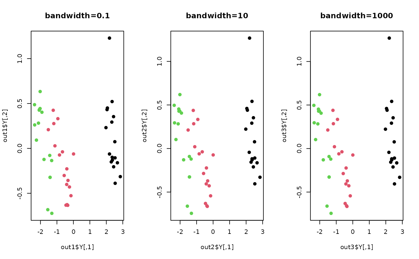
## use different kernel bandwidth
out1 <- do.kudp(X, bandwidth=0.1)
out2 <- do.kudp(X, bandwidth=10)
out3 <- do.kudp(X, bandwidth=1000)

## visualize
opar <- par(no.readonly=TRUE)
par(mfrow=c(1,3))
plot(out1$Y, col=lab, pch=19, main="bandwidth=0.1")
plot(out2$Y, col=lab, pch=19, main="bandwidth=10")
plot(out3$Y, col=lab, pch=19, main="bandwidth=1000")

par(opar)