Unsupervised Discriminant Projection

Unsupervised Discriminant Projection (UDP) aims finding projection that balances local and global scatter. Even though the name contains the word Discriminant, this algorithm is unsupervised. The term there reflects its algorithmic tactic to discriminate distance points not in the neighborhood of each data point. It performs PCA as intermittent preprocessing for rank singularity issue. Authors clearly mentioned that it is inspired by Locality Preserving Projection, which minimizes the local scatter only.

do.udp(
  X,
  ndim = 2,
  type = c("proportion", 0.1),
  preprocess = c("center", "scale", "cscale", "decorrelate", "whiten")
)

Arguments

X: an \((n\times p)\) matrix or data frame whose rows are observations and columns represent independent variables.
ndim: an integer-valued target dimension.
type: a vector of neighborhood graph construction. Following types are supported; c("knn",k), c("enn",radius), and c("proportion",ratio). Default is c("proportion",0.1), connecting about 1/10 of nearest data points among all data points. See also aux.graphnbd for more details.
preprocess: an additional option for preprocessing the data. Default is "center". See also aux.preprocess for more details.

Value

a named list containing

Y: an \((n\times ndim)\) matrix whose rows are embedded observations.
trfinfo: a list containing information for out-of-sample prediction.
projection: a \((p\times ndim)\) whose columns are basis for projection.
interimdim: the number of PCA target dimension used in preprocessing.

References

Yang J, Zhang D, Yang J, Niu B (2007). “Globally Maximizing, Locally Minimizing: Unsupervised Discriminant Projection with Applications to Face and Palm Biometrics.” IEEE Transactions on Pattern Analysis and Machine Intelligence, 29(4), 650--664.

Author

Kisung You

Examples

## load iris data
data(iris)
set.seed(100)
subid = sample(1:150,50)
X     = as.matrix(iris[subid,1:4])
label = as.factor(iris[subid,5])

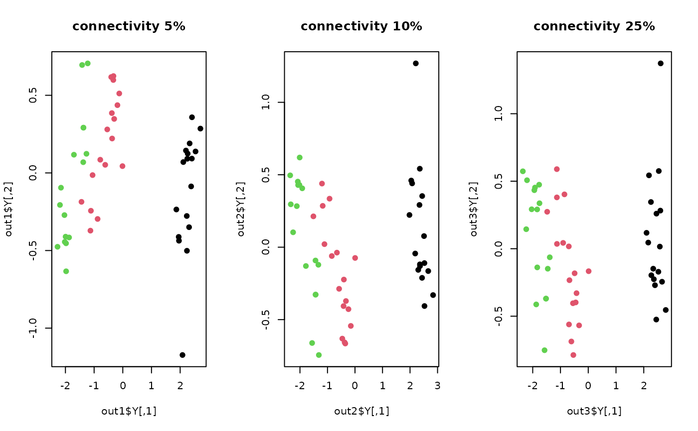
## use different connectivity level
out1 <- do.udp(X, type=c("proportion",0.05))
out2 <- do.udp(X, type=c("proportion",0.10))
out3 <- do.udp(X, type=c("proportion",0.25))

## visualize
opar <- par(no.readonly=TRUE)
par(mfrow=c(1,3))
plot(out1$Y, col=label, pch=19, main="connectivity 5%")
plot(out2$Y, col=label, pch=19, main="connectivity 10%")
plot(out3$Y, col=label, pch=19, main="connectivity 25%")

par(opar)