Sparse Subspace Clustering (SSC) assumes that the data points lie in
a union of low-dimensional subspaces. The algorithm constructs local
connectivity and uses the information for spectral clustering. SSC is
an implementation based on basis pursuit for sparse reconstruction for the
model without systematic noise, which solves
$$\textrm{min}_C \|C\|_1\quad\textrm{such that}\quad diag(C)=0,~D=DC$$
for column-stacked data matrix \(D\). If you are interested in
full implementation of the algorithm with sparse outliers and noise, please
contact the maintainer.
SSC(data, k = 2)
Arguments
| data | an \((n\times p)\) matrix of row-stacked observations. |
|---|---|
| k | the number of clusters (default: 2). |
Value
a named list of S3 class T4cluster containing
- cluster
a length-\(n\) vector of class labels (from \(1:k\)).
- algorithm
name of the algorithm.
References
Elhamifar E, Vidal R (2009). “Sparse Subspace Clustering.” In 2009 IEEE Conference on Computer Vision and Pattern Recognition, 2790--2797. ISBN 978-1-4244-3992-8.
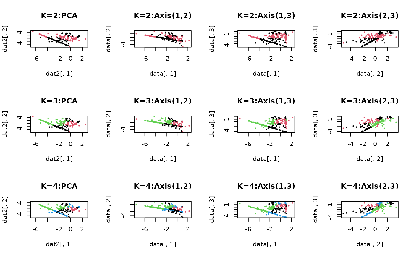
Examples
# \donttest{ ## generate a toy example set.seed(10) tester = genLP(n=100, nl=2, np=1, iso.var=0.1) data = tester$data label = tester$class ## do PCA for data reduction proj = base::eigen(stats::cov(data))$vectors[,1:2] dat2 = data%*%proj ## run SSC algorithm with k=2, 3, and 4 output2 = SSC(data, k=2) output3 = SSC(data, k=3) output4 = SSC(data, k=4) ## extract label information lab2 = output2$cluster lab3 = output3$cluster lab4 = output4$cluster ## visualize opar <- par(no.readonly=TRUE) par(mfrow=c(3,4)) plot(dat2[,1],dat2[,2],pch=19,cex=0.3,col=lab2,main="K=2:PCA") plot(data[,1],data[,2],pch=19,cex=0.3,col=lab2,main="K=2:Axis(1,2)") plot(data[,1],data[,3],pch=19,cex=0.3,col=lab2,main="K=2:Axis(1,3)") plot(data[,2],data[,3],pch=19,cex=0.3,col=lab2,main="K=2:Axis(2,3)") plot(dat2[,1],dat2[,2],pch=19,cex=0.3,col=lab3,main="K=3:PCA") plot(data[,1],data[,2],pch=19,cex=0.3,col=lab3,main="K=3:Axis(1,2)") plot(data[,1],data[,3],pch=19,cex=0.3,col=lab3,main="K=3:Axis(1,3)") plot(data[,2],data[,3],pch=19,cex=0.3,col=lab3,main="K=3:Axis(2,3)") plot(dat2[,1],dat2[,2],pch=19,cex=0.3,col=lab4,main="K=4:PCA") plot(data[,1],data[,2],pch=19,cex=0.3,col=lab4,main="K=4:Axis(1,2)") plot(data[,1],data[,3],pch=19,cex=0.3,col=lab4,main="K=4:Axis(1,3)") plot(data[,2],data[,3],pch=19,cex=0.3,col=lab4,main="K=4:Axis(2,3)")