This function generates a toy example of 'line and plane' data in \(R^3\) that data are generated from a mixture of lines (one-dimensional) planes (two-dimensional). The number of line- and plane-components are explicitly set by the user for flexible testing.
genLP(n = 100, nl = 1, np = 1, iso.var = 0.1)
Arguments
| n | the number of data points for each line and plane. |
|---|---|
| nl | the number of line components. |
| np | the number of plane components. |
| iso.var | degree of isotropic variance. |
Value
a named list containing with \(m = n\times(nl+np)\):
- data
an \((m\times 3)\) data matrix.
- class
length-\(m\) vector for class label.
- dimension
length-\(m\) vector of corresponding dimension from which an observation is created.
Examples
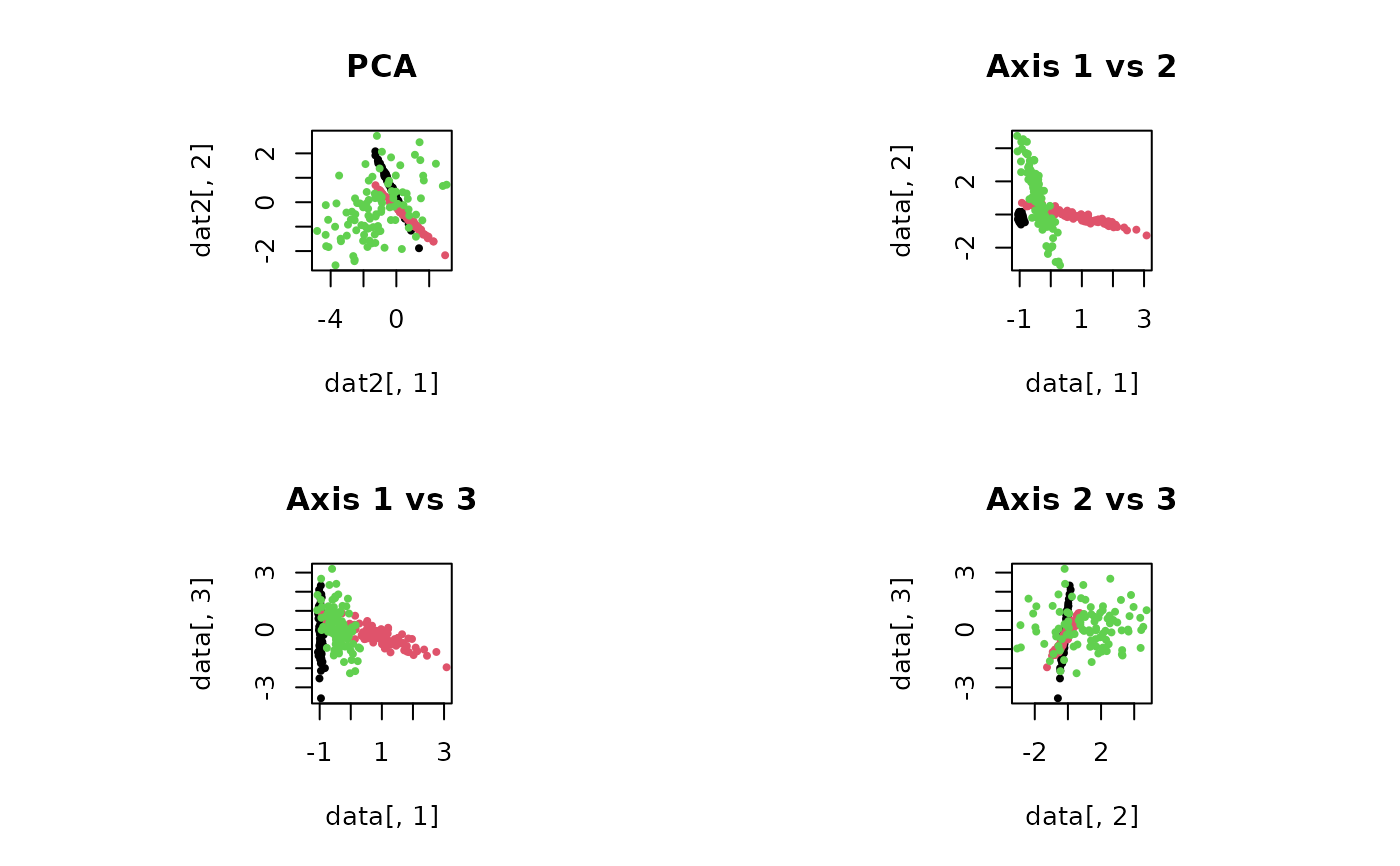
## test for visualization set.seed(10) tester = genLP(n=100, nl=1, np=2, iso.var=0.1) data = tester$data label = tester$class ## do PCA for data reduction proj = base::eigen(stats::cov(data))$vectors[,1:2] dat2 = data%*%proj ## visualize opar <- par(no.readonly=TRUE) par(mfrow=c(2,2), pty="s") plot(dat2[,1],dat2[,2],pch=19,cex=0.5,col=label,main="PCA") plot(data[,1],data[,2],pch=19,cex=0.5,col=label,main="Axis 1 vs 2") plot(data[,1],data[,3],pch=19,cex=0.5,col=label,main="Axis 1 vs 3") plot(data[,2],data[,3],pch=19,cex=0.5,col=label,main="Axis 2 vs 3")par(opar) if (FALSE) { ## visualize in 3d x11() scatterplot3d::scatterplot3d(x=data, pch=19, cex.symbols=0.5, color=label) }