Bayesian Mixture of Subspaces of Different Dimensions

MSM is a Bayesian model inferring mixtures of subspaces that are of possibly different dimensions. For simplicity, this function returns only a handful of information that are most important in representing the mixture model, including projection, location, and hard assignment parameters.

MSM(data, k = 2, ...)

Arguments

data	an \((n\times p)\) matrix of row-stacked observations.
k	the number of mixtures.
...	extra parameters including temperature temperature value for Gibbs posterior (default: 1e-6). prop.var proposal variance parameter (default: 1.0). iter the number of MCMC runs (default: 496). burn.in burn-in for MCMC runs (default: iter/2). thin interval for recording MCMC runs (default: 10). print.progress a logical; TRUE to show completion of iterations by 10, FALSE otherwise (default: FALSE).

Value

a list whose elements are S3 class "MSM" instances, which are also lists of following elements:

P

length-k list of projection matrices.

U

length-k list of orthonormal basis.

theta

length-k list of center locations of each mixture.

cluster

length-n vector of cluster label.

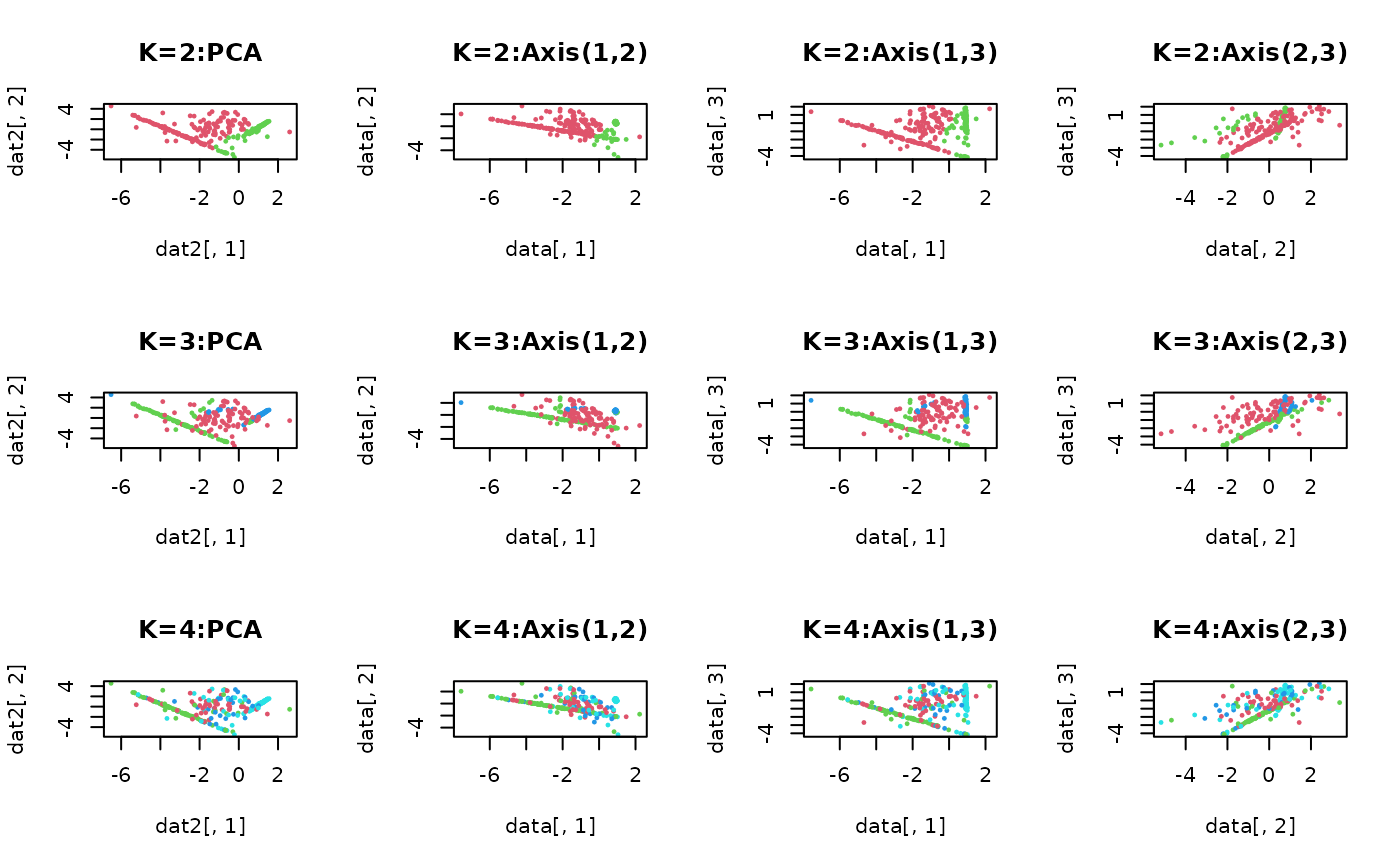
Examples

# \donttest{
## generate a toy example
set.seed(10)
tester = genLP(n=100, nl=2, np=1, iso.var=0.1)
data   = tester$data
label  = tester$class

## do PCA for data reduction
proj = base::eigen(stats::cov(data))$vectors[,1:2]
dat2 = data%*%proj

## run MSM algorithm with k=2, 3, and 4
maxiter = 500
output2 = MSM(data, k=2, iter=maxiter)
output3 = MSM(data, k=3, iter=maxiter)
output4 = MSM(data, k=4, iter=maxiter)

## extract final clustering information
nrec  = length(output2)
finc2 = output2[[nrec]]$cluster
finc3 = output3[[nrec]]$cluster
finc4 = output4[[nrec]]$cluster

## visualize
opar <- par(no.readonly=TRUE)
par(mfrow=c(3,4))
plot(dat2[,1],dat2[,2],pch=19,cex=0.3,col=finc2+1,main="K=2:PCA")
plot(data[,1],data[,2],pch=19,cex=0.3,col=finc2+1,main="K=2:Axis(1,2)")
plot(data[,1],data[,3],pch=19,cex=0.3,col=finc2+1,main="K=2:Axis(1,3)")
plot(data[,2],data[,3],pch=19,cex=0.3,col=finc2+1,main="K=2:Axis(2,3)")

plot(dat2[,1],dat2[,2],pch=19,cex=0.3,col=finc3+1,main="K=3:PCA")
plot(data[,1],data[,2],pch=19,cex=0.3,col=finc3+1,main="K=3:Axis(1,2)")
plot(data[,1],data[,3],pch=19,cex=0.3,col=finc3+1,main="K=3:Axis(1,3)")
plot(data[,2],data[,3],pch=19,cex=0.3,col=finc3+1,main="K=3:Axis(2,3)")

plot(dat2[,1],dat2[,2],pch=19,cex=0.3,col=finc4+1,main="K=4:PCA")
plot(data[,1],data[,2],pch=19,cex=0.3,col=finc4+1,main="K=4:Axis(1,2)")
plot(data[,1],data[,3],pch=19,cex=0.3,col=finc4+1,main="K=4:Axis(1,3)")
plot(data[,2],data[,3],pch=19,cex=0.3,col=finc4+1,main="K=4:Axis(2,3)")
par(opar)
# }