Low-Rank Representation (LRR) constructs the connectivity of the data by solving $$\textrm{min}_C \|C\|_*\quad\textrm{such that}\quad D=DC$$ for column-stacked data matrix \(D\) and \(\|\cdot \|_*\) is the nuclear norm which is relaxation of the rank condition. If you are interested in full implementation of the algorithm with sparse outliers and noise, please contact the maintainer.
LRR(data, k = 2, rank = 2)
Arguments
| data | an \((n\times p)\) matrix of row-stacked observations. |
|---|---|
| k | the number of clusters (default: 2). |
| rank | sum of dimensions for all \(k\) subspaces (default: 2). |
Value
a named list of S3 class T4cluster containing
- cluster
a length-\(n\) vector of class labels (from \(1:k\)).
- algorithm
name of the algorithm.
References
Liu G, Lin Z, Yu Y (2010). “Robust Subspace Segmentation by Low-Rank Representation.” In Proceedings of the 27th International Conference on International Conference on Machine Learning, ICML'10, 663--670. ISBN 978-1-60558-907-7.
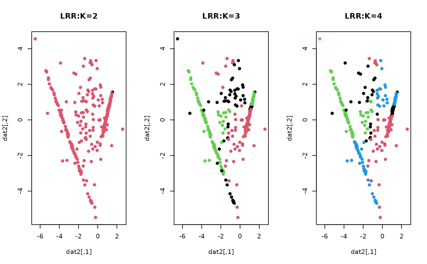
Examples
# \donttest{ ## generate a toy example set.seed(10) tester = genLP(n=100, nl=2, np=1, iso.var=0.1) data = tester$data label = tester$class ## do PCA for data reduction proj = base::eigen(stats::cov(data))$vectors[,1:2] dat2 = data%*%proj ## run LRR algorithm with k=2, 3, and 4 with rank=4 output2 = LRR(data, k=2, rank=4) output3 = LRR(data, k=3, rank=4) output4 = LRR(data, k=4, rank=4) ## extract label information lab2 = output2$cluster lab3 = output3$cluster lab4 = output4$cluster ## visualize opar <- par(no.readonly=TRUE) par(mfrow=c(1,3)) plot(dat2, pch=19, cex=0.9, col=lab2, main="LRR:K=2") plot(dat2, pch=19, cex=0.9, col=lab3, main="LRR:K=3") plot(dat2, pch=19, cex=0.9, col=lab4, main="LRR:K=4")