Supervised Laplacian Eigenmaps

Supervised Laplacian Eigenmaps (SPLAPEIG) is a supervised variant of Laplacian Eigenmaps. Instead of setting up explicit neighborhood, it utilizes an adaptive threshold strategy to define neighbors for both within- and between-class neighborhood. It then builds affinity matrices for each information and solves generalized eigenvalue problem. This algorithm may be quite sensitive in the choice of beta value.

do.splapeig(
  X,
  label,
  ndim = 2,
  preprocess = c("null", "center", "scale", "cscale", "whiten", "decorrelate"),
  beta = 1,
  gamma = 0.5
)

Arguments

X

an \((n\times p)\) matrix or data frame whose rows are observations and columns represent independent variables.

label

a length-\(n\) vector of data class labels.

ndim

an integer-valued target dimension.

preprocess

an additional option for preprocessing the data. Default is "null". See also aux.preprocess for more details.

beta

bandwidth parameter for heat kernel in \([0,\infty)\).

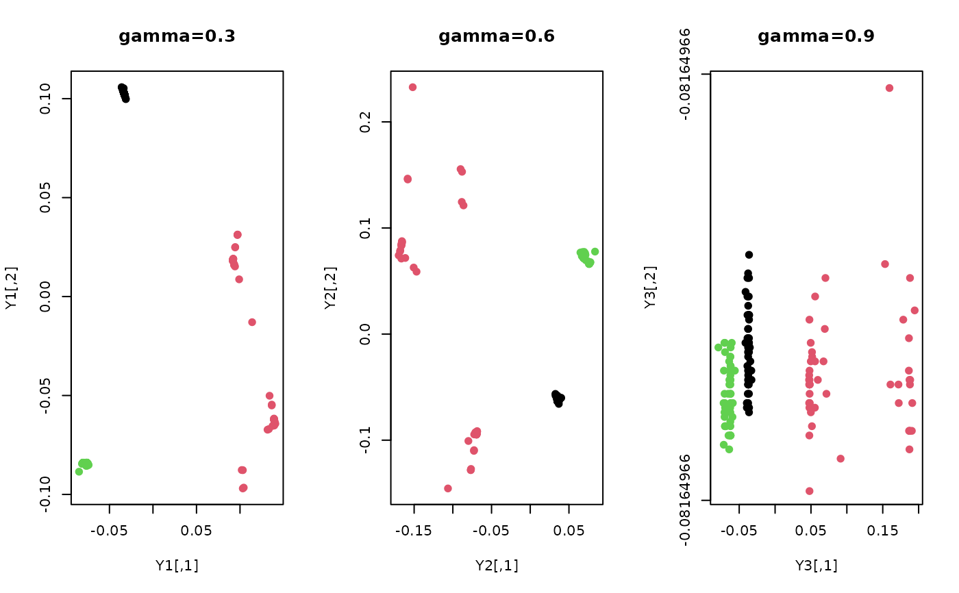
gamma

a balancing parameter in \([0,1]\) between within- and between-class information.

Value

a named list containing

Y

an \((n\times ndim)\) matrix whose rows are embedded observations.

trfinfo

a list containing information for out-of-sample prediction.

References

Raducanu B, Dornaika F (2012). “A Supervised Non-Linear Dimensionality Reduction Approach for Manifold Learning.” Pattern Recognition, 45(6), 2432--2444.

See also

do.lapeig

Author

Kisung You

Examples

# \donttest{
## load iris data
data(iris)
X     = as.matrix(iris[,1:4])
label = as.factor(iris[,5])

## try different balancing parameters with beta=50
out1 = do.splapeig(X, label, beta=50, gamma=0.3); Y1=out1$Y
out2 = do.splapeig(X, label, beta=50, gamma=0.6); Y2=out2$Y
out3 = do.splapeig(X, label, beta=50, gamma=0.9); Y3=out3$Y

## visualize
opar <- par(no.readonly=TRUE)
par(mfrow=c(1,3))
plot(Y1, pch=19, col=label, main="gamma=0.3")
plot(Y2, pch=19, col=label, main="gamma=0.6")
plot(Y3, pch=19, col=label, main="gamma=0.9")
#> Warning: relative range of values (  83 * EPS) is small (axis 2)

par(opar)
# }