Laplacian Eigenmaps

do.lapeig performs Laplacian Eigenmaps (LE) to discover low-dimensional manifold embedded in high-dimensional data space using graph laplacians. This is a classic algorithm employing spectral graph theory.

do.lapeig(X, ndim = 2, ...)

Arguments

X

an \((n\times p)\) matrix or data frame whose rows are observations and columns represent independent variables.

ndim

an integer-valued target dimension.

...

extra parameters including

kernelscale

kernel scale parameter. Default value is 1.0.

preprocess

an additional option for preprocessing the data. Default is "null". See also aux.preprocess for more details.

symmetric

one of "intersect", "union" or "asymmetric" is supported. Default is "union". See also aux.graphnbd for more details.

type

a vector of neighborhood graph construction. Following types are supported; c("knn",k), c("enn",radius), and c("proportion",ratio). Default is c("proportion",0.1), connecting about 1/10 of nearest data points among all data points. See also aux.graphnbd for more details.

weighted

a logical; TRUE for weighted graph laplacian and FALSE for combinatorial laplacian where connectivity is represented as 1 or 0 only.

Value

a named list containing

Y

an \((n\times ndim)\) matrix whose rows are embedded observations.

eigvals

a vector of eigenvalues for laplacian matrix.

trfinfo

a list containing information for out-of-sample prediction.

algorithm

name of the algorithm.

References

Belkin M, Niyogi P (2003). “Laplacian Eigenmaps for Dimensionality Reduction and Data Representation.” Neural Computation, 15(6), 1373--1396.

Author

Kisung You

Examples

# \donttest{
## use iris data
data(iris)
set.seed(100)
subid = sample(1:150,50)
X     = as.matrix(iris[subid,1:4])
lab   = as.factor(iris[subid,5])

## try different levels of connectivity
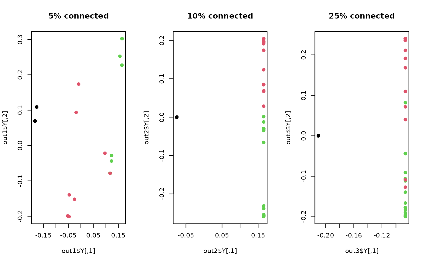
out1 <- do.lapeig(X, type=c("proportion",0.5), weighted=FALSE)
out2 <- do.lapeig(X, type=c("proportion",0.10), weighted=FALSE)
out3 <- do.lapeig(X, type=c("proportion",0.25), weighted=FALSE)

## Visualize
opar <- par(no.readonly=TRUE)
par(mfrow=c(1,3))
plot(out1$Y, pch=19, col=lab, main="5% connected")
plot(out2$Y, pch=19, col=lab, main="10% connected")
plot(out3$Y, pch=19, col=lab, main="25% connected")

par(opar)
# }