Nearest Neighbor Projection

Nearest Neighbor Projection is an iterative method for visualizing high-dimensional dataset in that a data is sequentially located in the low-dimensional space by maintaining the triangular distance spread of target data with its two nearest neighbors in the high-dimensional space. We extended the original method to be applied for arbitrarily low-dimensional space. Due the generalization, we opted for a global optimization method of Differential Evolution (DEoptim) within in that it may add computational burden to certain degrees.

do.nnp(
  X,
  ndim = 2,
  preprocess = c("null", "center", "scale", "cscale", "whiten", "decorrelate")
)

Arguments

X

an \((n\times p)\) matrix or data frame whose rows are observations and columns represent independent variables.

ndim

an integer-valued target dimension.

preprocess

an additional option for preprocessing the data. Default is "null". See also aux.preprocess for more details.

Value

a named list containing

Y

an \((n\times ndim)\) matrix whose rows are embedded observations.

trfinfo

a list containing information for out-of-sample prediction.

References

Tejada E, Minghim R, Nonato LG (2003). “On Improved Projection Techniques to Support Visual Exploration of Multidimensional Data Sets.” Information Visualization, 2(4), 218--231.

Author

Kisung You

Examples

# \donttest{
## use iris data
data(iris)
set.seed(100)
subid = sample(1:150,50)
X     = as.matrix(iris[subid,1:4])
label = as.factor(iris[subid,5])

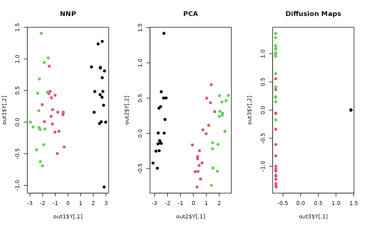
## let's compare with other methods
out1 <- do.nnp(X, ndim=2)      # NNP
out2 <- do.pca(X, ndim=2)      # PCA
out3 <- do.dm(X, ndim=2)     # Diffusion Maps

## visualize
opar <- par(no.readonly=TRUE)
par(mfrow=c(1,3))
plot(out1$Y, pch=19, col=label, main="NNP")
plot(out2$Y, pch=19, col=label, main="PCA")
plot(out3$Y, pch=19, col=label, main="Diffusion Maps")

par(opar)
# }