Maximum Variance Unfolding / Semidefinite Embedding

The method of Maximum Variance Unfolding(MVU), also known as Semidefinite Embedding(SDE) is, as its names suggest, to exploit semidefinite programming in performing nonlinear dimensionality reduction by unfolding neighborhood graph constructed in the original high-dimensional space. Its unfolding generates a gram matrix \(K\) in that we can choose from either directly finding embeddings ("spectral") or use again Kernel PCA technique ("kpca") to find low-dimensional representations.

do.mvu(
  X,
  ndim = 2,
  type = c("proportion", 0.1),
  preprocess = c("null", "center", "scale", "cscale", "decorrelate", "whiten"),
  projtype = c("spectral", "kpca")
)

Arguments

X

an \((n\times p)\) matrix or data frame whose rows are observations and columns represent independent variables.

ndim

an integer-valued target dimension.

type

a vector of neighborhood graph construction. Following types are supported; c("knn",k), c("enn",radius), and c("proportion",ratio). Default is c("proportion",0.1), connecting about 1/10 of nearest data points among all data points. See also aux.graphnbd for more details.

preprocess

an additional option for preprocessing the data. Default is "null". See also aux.preprocess for more details.

projtype

type of method for projection; either "spectral" or "kpca" used.

Value

a named list containing

Y

an \((n\times ndim)\) matrix whose rows are embedded observations.

trfinfo

a list containing information for out-of-sample prediction.

References

Weinberger KQ, Saul LK (2006). “Unsupervised Learning of Image Manifolds by Semidefinite Programming.” International Journal of Computer Vision, 70(1), 77--90.

Author

Kisung You

Examples

# \donttest{
## use a small subset of iris data
set.seed(100)
id  = sample(1:150, 50)
X   = as.matrix(iris[id,1:4])
lab = as.factor(iris[id,5])

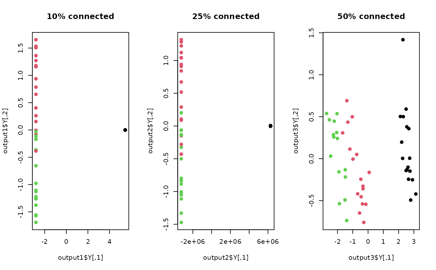
## try different connectivity levels
output1 <- do.mvu(X, type=c("proportion", 0.10))
output2 <- do.mvu(X, type=c("proportion", 0.25))
output3 <- do.mvu(X, type=c("proportion", 0.50))

## visualize three different projections
opar <- par(no.readonly=TRUE)
par(mfrow=c(1,3))
plot(output1$Y, main="10% connected", pch=19, col=lab)
plot(output2$Y, main="25% connected", pch=19, col=lab)
plot(output3$Y, main="50% connected", pch=19, col=lab)

par(opar)
# }