Landmark Isometric Feature Mapping

Landmark Isomap is a variant of Isomap in that it first finds a low-dimensional embedding using a small portion of given dataset and graft the others in a manner to preserve as much pairwise distance from all the other data points to landmark points as possible.

do.lisomap(
  X,
  ndim = 2,
  ltype = c("random", "MaxMin"),
  npoints = max(nrow(X)/5, ndim + 1),
  preprocess = c("center", "scale", "cscale", "decorrelate", "whiten"),
  type = c("proportion", 0.1),
  symmetric = c("union", "intersect", "asymmetric"),
  weight = TRUE
)

Arguments

X

an \((n\times p)\) matrix or data frame whose rows are observations and columns represent independent variables.

ndim

an integer-valued target dimension.

ltype

on how to select landmark points, either "random" or "MaxMin".

npoints

the number of landmark points to be drawn.

preprocess

an option for preprocessing the data. Default is "center". See also aux.preprocess for more details.

type

a vector of neighborhood graph construction. Following types are supported; c("knn",k), c("enn",radius), and c("proportion",ratio). Default is c("proportion",0.1), connecting about 1/10 of nearest data points among all data points. See also aux.graphnbd for more details.

symmetric

one of "intersect", "union" or "asymmetric" is supported. Default is "union". See also aux.graphnbd for more details.

weight

TRUE to perform Landmark Isomap on weighted graph, or FALSE otherwise.

Value

a named list containing

Y

an \((n\times ndim)\) matrix whose rows are embedded observations.

trfinfo

a list containing information for out-of-sample prediction.

References

Silva VD, Tenenbaum JB (2003). “Global Versus Local Methods in Nonlinear Dimensionality Reduction.” In Becker S, Thrun S, Obermayer K (eds.), Advances in Neural Information Processing Systems 15, 721--728. MIT Press.

See also

do.isomap

Author

Kisung You

Examples

# \donttest{
## use iris data
data(iris)
X   <- as.matrix(iris[,1:4])
lab <- as.factor(iris[,5])

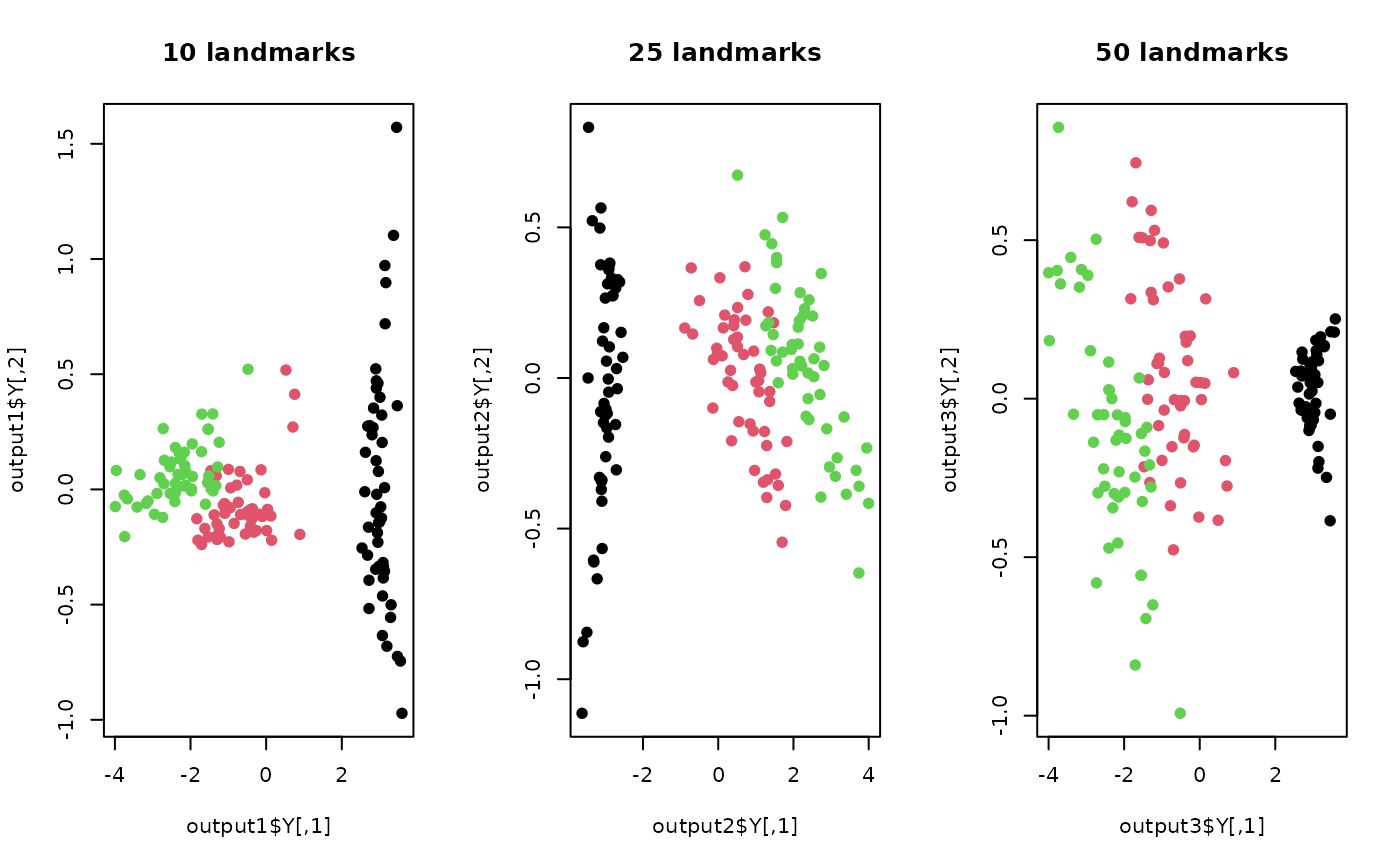
## use different number of data points as landmarks
output1 <- do.lisomap(X, npoints=10, type=c("proportion",0.25))
output2 <- do.lisomap(X, npoints=25, type=c("proportion",0.25))
output3 <- do.lisomap(X, npoints=50, type=c("proportion",0.25))

## visualize three different projections
opar <- par(no.readonly=TRUE)
par(mfrow=c(1,3))
plot(output1$Y, pch=19, col=lab, main="10 landmarks")
plot(output2$Y, pch=19, col=lab, main="25 landmarks")
plot(output3$Y, pch=19, col=lab, main="50 landmarks")

par(opar)
# }