The isometric SPE (ISPE) adopts the idea of approximating geodesic distance on embedded manifold
when two data points are close enough. It introduces the concept of cutoff where the learning process
is only applied to the pair of data points whose original proximity is small enough to be considered as
mutually local whose distance should be close to geodesic distance.
do.ispe(
  X,
  ndim = 2,
  proximity = function(x) {
     dist(x, method = "euclidean")
 },
  C = 50,
  S = 50,
  lambda = 1,
  drate = 0.9,
  cutoff = 1
)
Arguments
- X
an \((n\times p)\) matrix or data frame whose rows are observations and columns represent independent variables.
- ndim
an integer-valued target dimension.
- proximity
a function for constructing proximity matrix from original data dimension.
- C
the number of cycles to be run; after each cycle, learning parameter
- S
the number of updates for each cycle.
- lambda
initial learning parameter.
- drate
multiplier for
lambdaat each cycle; should be a positive real number in \((0,1).\)- cutoff
cutoff threshold value.
Value
a named list containing
- Y
an \((n\times ndim)\) matrix whose rows are embedded observations.
- trfinfo
a list containing information for out-of-sample prediction.
References
Agrafiotis DK, Xu H (2002). “A Self-Organizing Principle for Learning Nonlinear Manifolds.” Proceedings of the National Academy of Sciences, 99(25), 15869–15872.
Examples
## load iris data
data(iris)
set.seed(100)
subid = sample(1:150,50)
X = as.matrix(iris[subid,1:4])
label = as.factor(iris[subid,5])
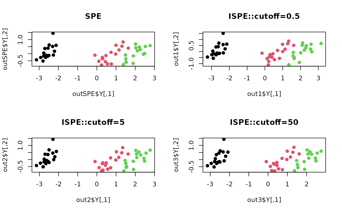
## compare with original SPE
outSPE <- do.spe(X, ndim=2)
out1 <- do.ispe(X, ndim=2, cutoff=0.5)
out2 <- do.ispe(X, ndim=2, cutoff=5)
out3 <- do.ispe(X, ndim=2, cutoff=50)
## Visualize
opar <- par(no.readonly=TRUE)
par(mfrow=c(2,2))
plot(outSPE$Y, pch=19, col=label, main="SPE")
plot(out1$Y, pch=19, col=label, main="ISPE::cutoff=0.5")
plot(out2$Y, pch=19, col=label, main="ISPE::cutoff=5")
plot(out3$Y, pch=19, col=label, main="ISPE::cutoff=50")
 par(opar)