Stochastic Proximity Embedding

One of drawbacks for Multidimensional Scaling or Sammon mapping is that they have quadratic computational complexity with respect to the number of data. Stochastic Proximity Embedding (SPE) adopts stochastic update rule in that its computational speed is much improved. It performs C number of cycles, where for each cycle, it randomly selects two data points and updates their locations correspondingly S times. After each cycle, learning parameter \(\lambda\) is multiplied by drate, becoming smaller in magnitude.

do.spe(
  X,
  ndim = 2,
  proximity = function(x) {
     dist(x, method = "euclidean")
 },
  C = 50,
  S = 50,
  lambda = 1,
  drate = 0.9
)

Arguments

X

an \((n\times p)\) matrix or data frame whose rows are observations and columns represent independent variables.

ndim

an integer-valued target dimension.

proximity

a function for constructing proximity matrix from original data dimension.

C

the number of cycles to be run; after each cycle, learning parameter

S

the number of updates for each cycle.

lambda

initial learning parameter.

drate

multiplier for lambda at each cycle; should be a positive real number in \((0,1).\)

Value

a named list containing

Y

an \((n\times ndim)\) matrix whose rows are embedded observations.

trfinfo

a list containing information for out-of-sample prediction.

References

Agrafiotis DK (2003). “Stochastic Proximity Embedding.” Journal of Computational Chemistry, 24(10), 1215--1221.

Author

Kisung You

Examples

# \donttest{
## load iris data
data(iris)
X     = as.matrix(iris[,1:4])
label = as.factor(iris$Species)

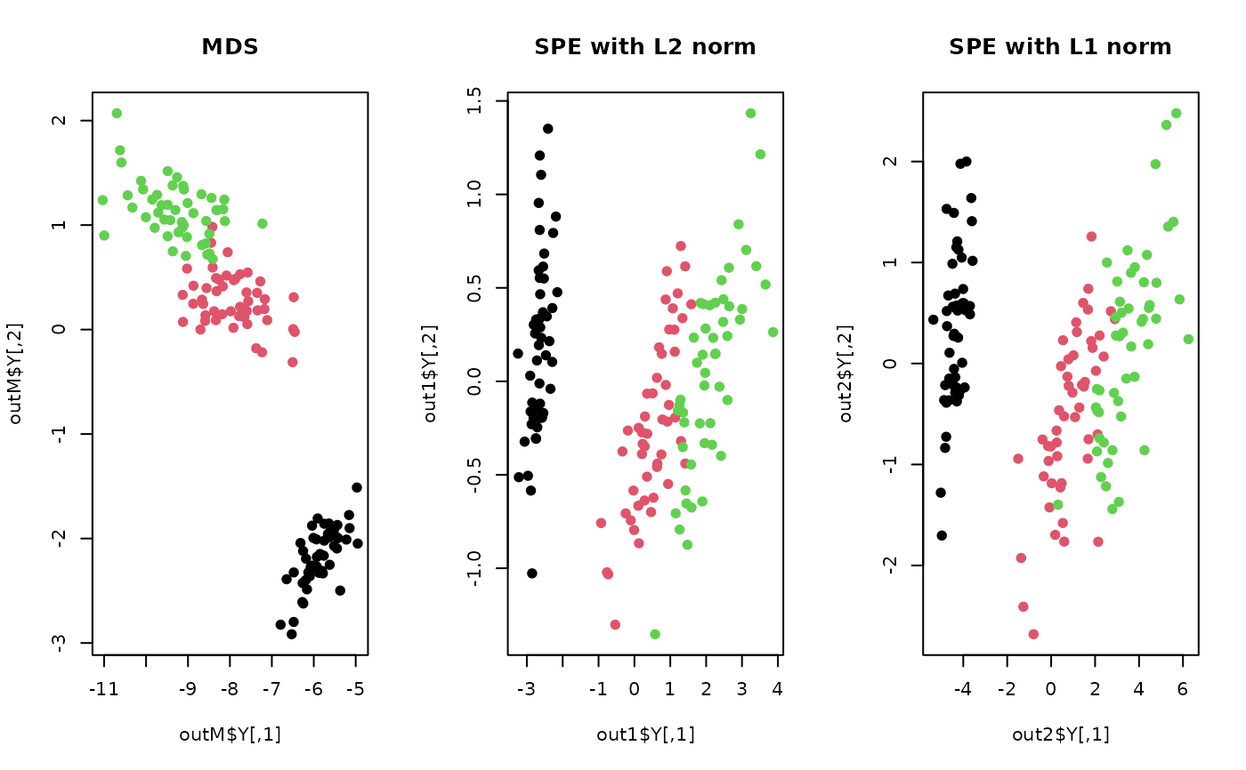
## compare with mds using 2 distance metrics
outM <- do.mds(X, ndim=2)
out1 <- do.spe(X, ndim=2)
out2 <- do.spe(X, ndim=2, proximity=function(x){dist(x, method="manhattan")})

## Visualize
opar <- par(no.readonly=TRUE)
par(mfrow=c(1,3))
plot(outM$Y, pch=19, col=label, main="MDS")
plot(out1$Y, pch=19, col=label, main="SPE with L2 norm")
plot(out2$Y, pch=19, col=label, main="SPE with L1 norm")

par(opar)
# }