Dual view of PPCA optimizes the latent variables directly from a simple Bayesian approach to model the noise using the multivariate Gaussian distribution of zero mean and spherical covariance \(\beta^{-1} I\). When \(\beta\) is too small, the algorithm automatically returns an error and provides a guideline for minimal value that enables successful computation.
do.dppca(X, ndim = 2, beta = 1)Arguments
Value
a named Rdimtools S3 object containing
- Y
an \((n\times ndim)\) matrix whose rows are embedded observations.
- algorithm
name of the algorithm.
References
Lawrence N (2005). “Probabilistic Non-linear Principal Component Analysis with Gaussian Process Latent Variable Models.” Journal of Machine Learning Research, 6(60), 1783-1816.
See also
Examples
# \donttest{
## load iris data
data(iris)
X = as.matrix(iris[,1:4])
lab = as.factor(iris[,5])
## compare difference choices of 'beta'
embed1 <- do.dppca(X, beta=0.2)
#> [1] 157.502004 9.039485
embed2 <- do.dppca(X, beta=1)
#> [1] 157.502004 9.039485
embed3 <- do.dppca(X, beta=5)
#> [1] 157.502004 9.039485
## Visualize
opar <- par(no.readonly=TRUE)
par(mfrow=c(1,3), pty="s")
plot(embed1$Y , col=lab, pch=19, main="beta=0.2")
plot(embed2$Y , col=lab, pch=19, main="beta=1")
plot(embed3$Y , col=lab, pch=19, main="beta=5")
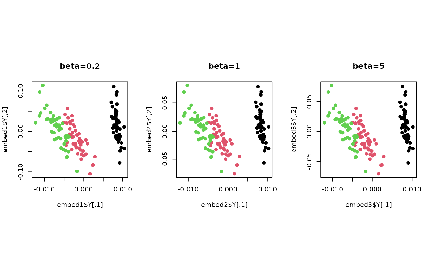 par(opar)
# }
par(opar)
# }