Probabilistic PCA (PPCA) is a probabilistic framework to explain the well-known PCA model. Using the conjugacy of normal model, we compute MLE for values explicitly derived in the paper. Note that unlike PCA where loadings are directly used for projection, PPCA uses \(WM^{-1}\) as projection matrix, as it is relevant to the error model. Also, for high-dimensional problem, it is possible that MLE can have negative values if sample covariance given the data is rank-deficient.
do.ppca(X, ndim = 2)Arguments
Value
a named Rdimtools S3 object containing
- Y
an \((n\times ndim)\) matrix whose rows are embedded observations.
- projection
a \((p\times ndim)\) whose columns are basis for projection.
- mle.sigma2
MLE for \(\sigma^2\).
- mle.W
MLE of a \((p\times ndim)\) mapping from latent to observation in column major.
- algorithm
name of the algorithm.
References
Tipping ME, Bishop CM (1999). “Probabilistic Principal Component Analysis.” Journal of the Royal Statistical Society: Series B (Statistical Methodology), 61(3), 611–622.
See also
Examples
# \donttest{
## use iris data
data(iris)
set.seed(100)
subid = sample(1:150, 50)
X = as.matrix(iris[subid,1:4])
label = as.factor(iris[subid,5])
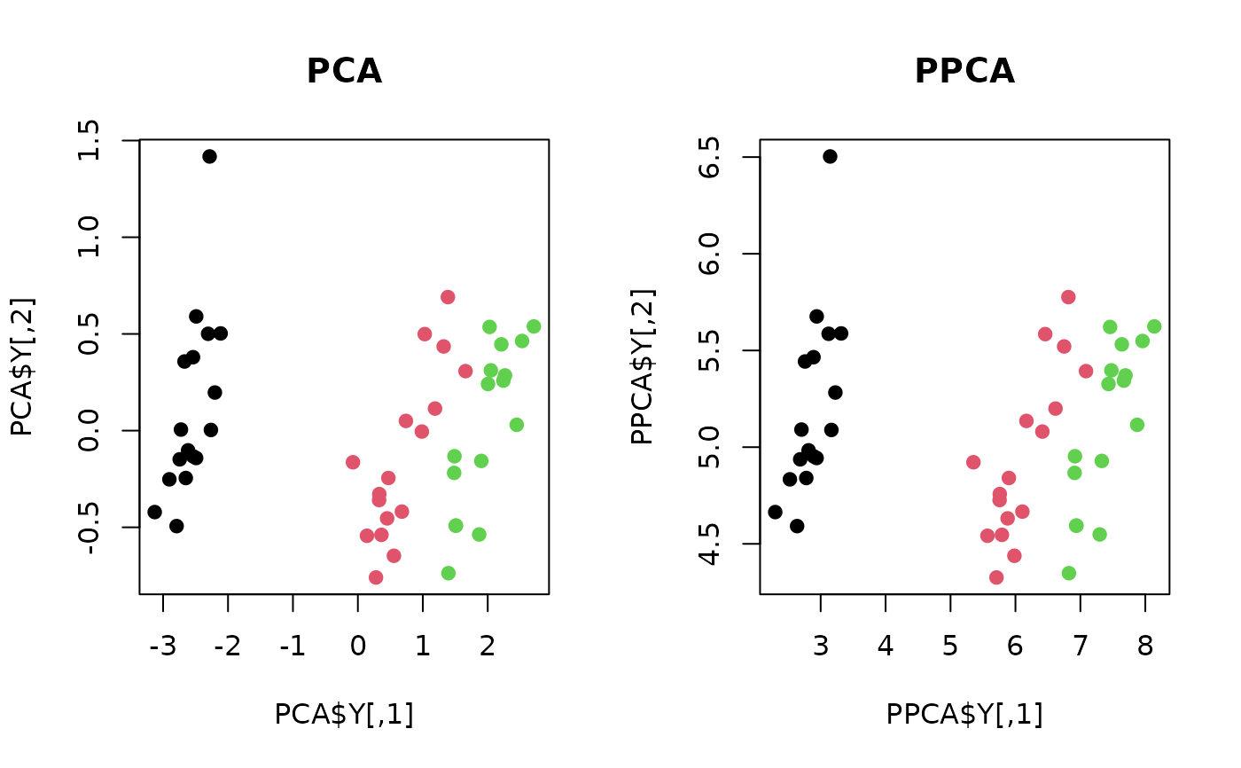
## Compare PCA and PPCA
PCA <- do.pca(X, ndim=2)
PPCA <- do.ppca(X, ndim=2)
## Visualize
opar <- par(no.readonly=TRUE)
par(mfrow=c(1,2))
plot(PCA$Y, pch=19, col=label, main="PCA")
plot(PPCA$Y, pch=19, col=label, main="PPCA")
 par(opar)
# }
par(opar)
# }