Bayesian Multidimensional Scaling

A Bayesian formulation of classical Multidimensional Scaling is presented. Even though this method is based on MCMC sampling, we only return maximum a posterior (MAP) estimate that maximizes the posterior distribution. Due to its nature without any special tuning, increasing mc.iter requires much computation. A note on the method is that this algorithm does not return an explicit form of projection matrix so it's classified in our package as a nonlinear method. Also, automatic dimension selection is not supported for simplicity as well as consistency with other methods in the package.

do.bmds(
  X,
  ndim = 2,
  par.a = 5,
  par.alpha = 0.5,
  par.step = 1,
  mc.iter = 50,
  print.progress = FALSE
)

Arguments

X

an \((n\times p)\) matrix whose rows are observations and columns represent independent variables.

ndim

an integer-valued target dimension.

par.a

hyperparameter for conjugate prior on variance term, i.e., \(\sigma^2 \sim IG(a,b)\). Note that \(b\) is chosen appropriately as in paper.

par.alpha

hyperparameter for conjugate prior on diagonal term, i.e., \(\lambda_j \sim IG(\alpha, \beta_j)\). Note that \(\beta_j\) is chosen appropriately as in paper.

par.step

stepsize for random-walk, which is standard deviation of Gaussian proposal.

mc.iter

the number of MCMC iterations.

print.progress

a logical; TRUE to show iterations, FALSE otherwise (default: FALSE).

Value

a named Rdimtools S3 object containing

Y

an \((n\times ndim)\) matrix whose rows are embedded observations.

algorithm

name of the algorithm.

References

Oh M, Raftery AE (2001). “Bayesian Multidimensional Scaling and Choice of Dimension.” Journal of the American Statistical Association, 96(455), 1031--1044.

Author

Kisung You

Examples

# \donttest{
## load iris data
data(iris)
set.seed(100)
subid = sample(1:150,50)
X     = as.matrix(iris[subid,1:4])
label = as.factor(iris[subid,5])

## compare with other methods
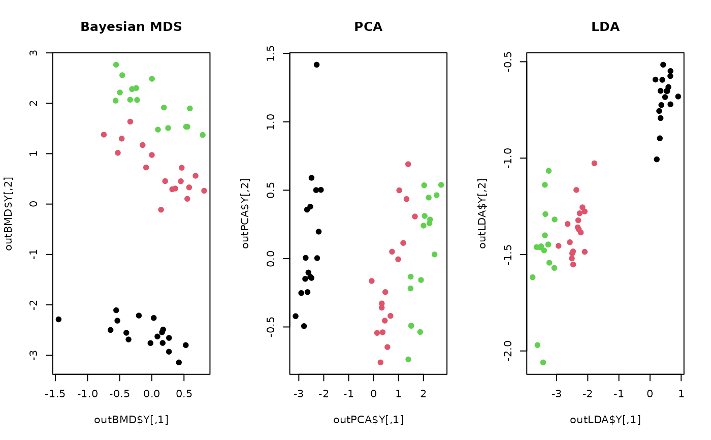
outBMD <- do.bmds(X, ndim=2)
outPCA <- do.pca(X, ndim=2)
outLDA <- do.lda(X, label, ndim=2)

## visualize
opar <- par(no.readonly=TRUE)
par(mfrow=c(1,3))
plot(outBMD$Y, pch=19, col=label, main="Bayesian MDS")
plot(outPCA$Y, pch=19, col=label, main="PCA")
plot(outLDA$Y, pch=19, col=label, main="LDA")

par(opar)
# }