Linear Discriminant Analysis (LDA) originally aims to find a set of features
that best separate groups of data. Since we need label information,
LDA belongs to a class of supervised methods of performing classification.
However, since it is based on finding suitable projections, it can still
be used to do dimension reduction. We support both binary and multiple-class cases.
Note that the target dimension ndim should be less than or equal to K-1,
where K is the number of classes, or K=length(unique(label)). Our code
automatically gives bounds on user's choice to correspond to what theory has shown. See
the comments section for more details.
do.lda(X, label, ndim = 2)Arguments
Value
a named Rdimtools S3 object containing
- Y
an \((n\times ndim)\) matrix whose rows are embedded observations.
- projection
a \((p\times ndim)\) whose columns are basis for projection.
- algorithm
name of the algorithm.
Limit of Target Dimension Selection
In unsupervised algorithms, selection of ndim is arbitrary as long as
the target dimension is lower-dimensional than original data dimension, i.e., ndim < p.
In LDA, it is not allowed. Suppose we have K classes, then its formulation on
\(S_B\), between-group variance, has maximum rank of K-1. Therefore, the maximal
subspace can only be spanned by at most K-1 orthogonal vectors.
References
Fisher RA (1936). “THE USE OF MULTIPLE MEASUREMENTS IN TAXONOMIC PROBLEMS.” Annals of Eugenics, 7(2), 179–188.
Fukunaga K (1990). Introduction to Statistical Pattern Recognition, Computer Science and Scientific Computing, 2nd ed edition. Academic Press, Boston. ISBN 978-0-12-269851-4.
Examples
# \donttest{
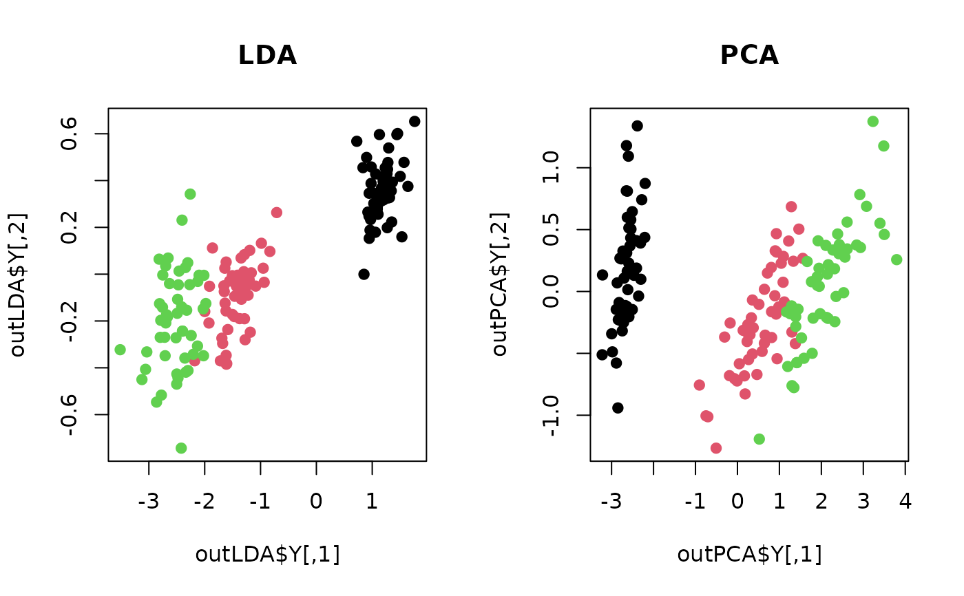
## use iris dataset
data(iris)
X = as.matrix(iris[,1:4])
lab = as.factor(iris[,5])
## compare with PCA
outLDA = do.lda(X, lab, ndim=2)
outPCA = do.pca(X, ndim=2)
## visualize
opar <- par(no.readonly=TRUE)
par(mfrow=c(1,2))
plot(outLDA$Y, col=lab, pch=19, main="LDA")
plot(outPCA$Y, col=lab, pch=19, main="PCA")
 par(opar)
# }
par(opar)
# }