Locality-Preserved Maximum Information Projection

Locality-Preserved Maximum Information Projection (LPMIP) is an unsupervised linear dimension reduction method to identify the underlying manifold structure by learning both the within- and between-locality information. The parameter alpha is balancing the tradeoff between two and the flexibility of this model enables an interpretation of it as a generalized extension of LPP.

do.lpmip(
  X,
  ndim = 2,
  type = c("proportion", 0.1),
  preprocess = c("null", "center", "scale", "cscale", "whiten", "decorrelate"),
  sigma = 10,
  alpha = 0.5
)

Arguments

X: an \((n\times p)\) matrix or data frame whose rows are observations and columns represent independent variables.
ndim: an integer-valued target dimension.
type: a vector of neighborhood graph construction. Following types are supported; c("knn",k), c("enn",radius), and c("proportion",ratio). Default is c("proportion",0.1), connecting about 1/10 of nearest data points among all data points. See also aux.graphnbd for more details.
preprocess: an additional option for preprocessing the data. Default is "null". See also aux.preprocess for more details.
sigma: bandwidth parameter for heat kernel in \((0,\infty)\).
alpha: balancing parameter between two locality information in \([0,1]\).

Value

a named list containing

Y: an \((n\times ndim)\) matrix whose rows are embedded observations.
trfinfo: a list containing information for out-of-sample prediction.
projection: a \((p\times ndim)\) whose columns are basis for projection.

References

Haixian Wang, Sibao Chen, Zilan Hu, Wenming Zheng (2008). “Locality-Preserved Maximum Information Projection.” IEEE Transactions on Neural Networks, 19(4), 571--585.

Author

Kisung You

Examples

## use iris dataset
data(iris)
set.seed(100)
subid <- sample(1:150, 50)
X     <- as.matrix(iris[subid,1:4])
lab   <- as.factor(iris[subid,5])

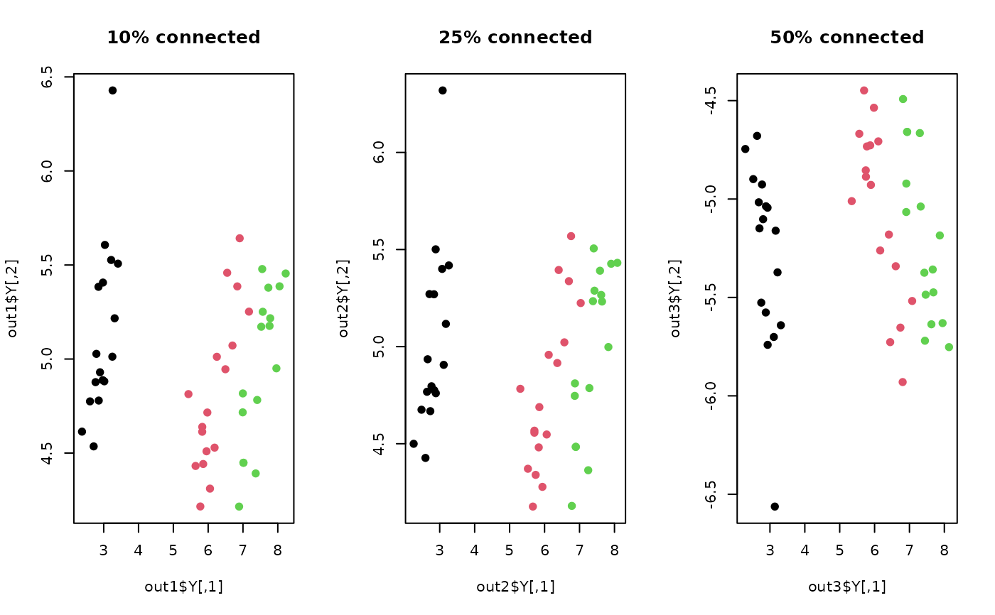
## try different neighborhood size
out1 <- do.lpmip(X, ndim=2, type=c("proportion",0.10))
out2 <- do.lpmip(X, ndim=2, type=c("proportion",0.25))
out3 <- do.lpmip(X, ndim=2, type=c("proportion",0.50))

## Visualize
opar <- par(no.readonly=TRUE)
par(mfrow=c(1,3))
plot(out1$Y, pch=19, col=lab, main="10% connected")
plot(out2$Y, pch=19, col=lab, main="25% connected")
plot(out3$Y, pch=19, col=lab, main="50% connected")

par(opar)