Locality Preserving Fisher Discriminant Analysis (LPFDA) is a supervised variant of LPP. It can also be seemed as an improved version of LDA where the locality structure of the data is preserved. The algorithm aims at getting a subspace projection matrix by solving a generalized eigenvalue problem.
Arguments
- X
an \((n\times p)\) matrix or data frame whose rows are observations and columns represent independent variables.
- label
a length-\(n\) vector of data class labels.
- ndim
an integer-valued target dimension.
- type
a vector of neighborhood graph construction. Following types are supported;
c("knn",k),c("enn",radius), andc("proportion",ratio). Default isc("proportion",0.1), connecting about 1/10 of nearest data points among all data points. See alsoaux.graphnbdfor more details.- preprocess
an additional option for preprocessing the data. Default is "center". See also
aux.preprocessfor more details.- t
bandwidth parameter for heat kernel in \((0,\infty)\).
Value
a named list containing
- Y
an \((n\times ndim)\) matrix whose rows are embedded observations.
- trfinfo
a list containing information for out-of-sample prediction.
- projection
a \((p\times ndim)\) whose columns are basis for projection.
References
Zhao X, Tian X (2009). “Locality Preserving Fisher Discriminant Analysis for Face Recognition.” In Huang D, Jo K, Lee H, Kang H, Bevilacqua V (eds.), Emerging Intelligent Computing Technology and Applications, 261--269.
Examples
## generate data of 3 types with clear difference
set.seed(100)
dt1 = aux.gensamples(n=20)-50
dt2 = aux.gensamples(n=20)
dt3 = aux.gensamples(n=20)+50
## merge the data and create a label correspondingly
X = rbind(dt1,dt2,dt3)
label = rep(1:3, each=20)
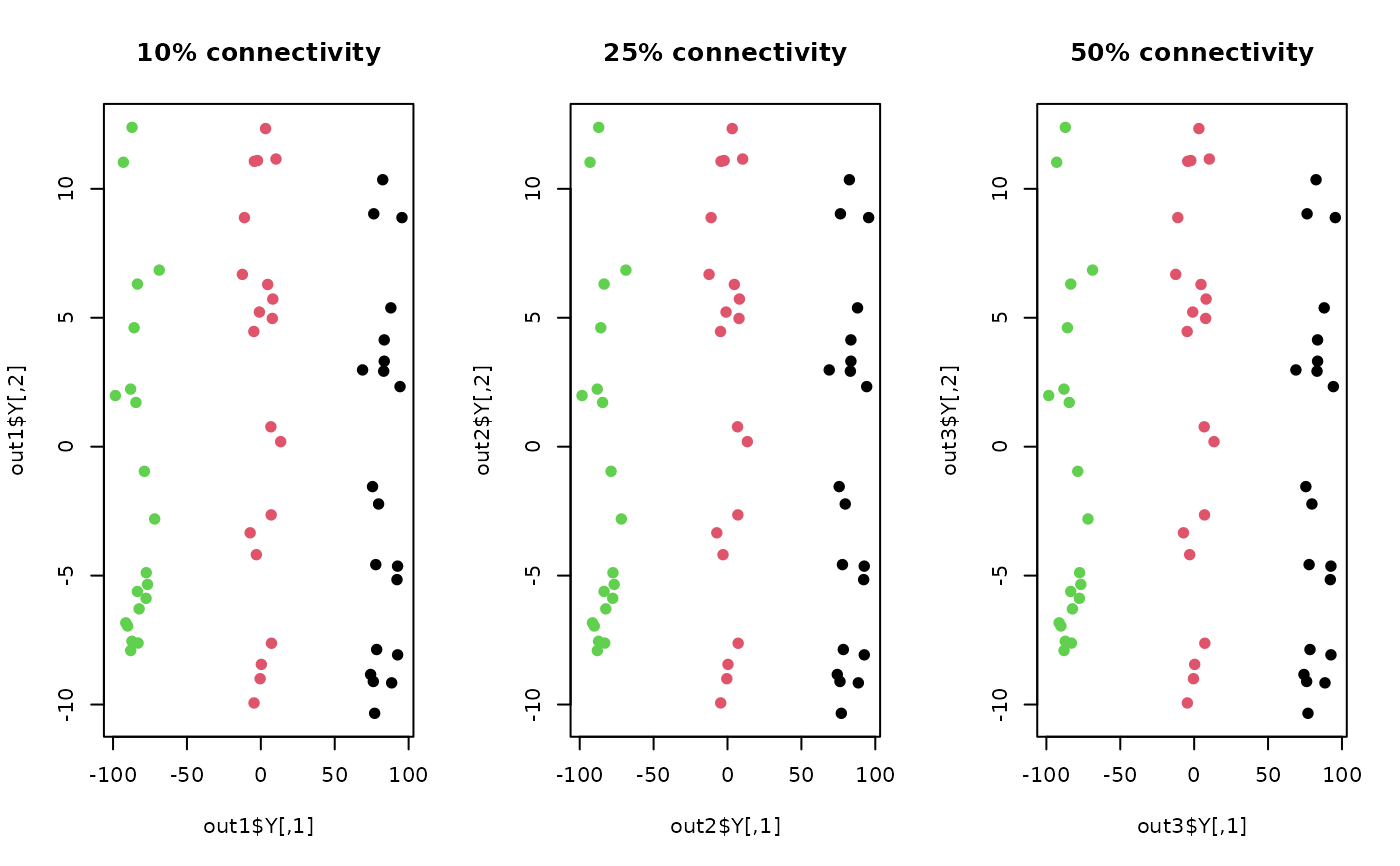
## try different proportion of connected edges
out1 = do.lpfda(X, label, type=c("proportion",0.10))
out2 = do.lpfda(X, label, type=c("proportion",0.25))
out3 = do.lpfda(X, label, type=c("proportion",0.50))
## visualize
opar <- par(no.readonly=TRUE)
par(mfrow=c(1,3))
plot(out1$Y, pch=19, col=label, main="10% connectivity")
plot(out2$Y, pch=19, col=label, main="25% connectivity")
plot(out3$Y, pch=19, col=label, main="50% connectivity")
 par(opar)