Linear Local Tangent Space Alignment

Linear Local Tangent Space Alignment (LLTSA) is a linear variant of the celebrated LTSA method. It uses the tangent space in the neighborhood for each data point to represent the local geometry. Alignment of those local tangent spaces in the low-dimensional space returns an explicit mapping from the high-dimensional space.

do.lltsa(
  X,
  ndim = 2,
  type = c("proportion", 0.1),
  symmetric = c("union", "intersect", "asymmetric"),
  preprocess = c("center", "scale", "cscale", "decorrelate", "whiten")
)

Arguments

X

an \((n\times p)\) matrix or data frame whose rows are observations and columns represent independent variables.

ndim

an integer-valued target dimension.

type

a vector of neighborhood graph construction. Following types are supported; c("knn",k), c("enn",radius), and c("proportion",ratio). Default is c("proportion",0.1), connecting about 1/10 of nearest data points among all data points. See also aux.graphnbd for more details.

symmetric

one of "intersect", "union" or "asymmetric" is supported. Default is "union". See also aux.graphnbd for more details.

preprocess

an additional option for preprocessing the data. Default is "center". See also aux.preprocess for more details.

Value

a named list containing

Y

an \((n\times ndim)\) matrix whose rows are embedded observations.

trfinfo

a list containing information for out-of-sample prediction.

projection

a \((p\times ndim)\) whose columns are basis for projection.

References

Zhang T, Yang J, Zhao D, Ge X (2007). “Linear Local Tangent Space Alignment and Application to Face Recognition.” Neurocomputing, 70(7-9), 1547--1553.

See also

do.ltsa

Author

Kisung You

Examples

## use iris dataset
data(iris)
set.seed(100)
subid = sample(1:150,50)
X     = as.matrix(iris[subid,1:4])
lab   = as.factor(iris[subid,5])

## try different neighborhood size
out1 <- do.lltsa(X, type=c("proportion",0.25))
out2 <- do.lltsa(X, type=c("proportion",0.50))
out3 <- do.lltsa(X, type=c("proportion",0.75))

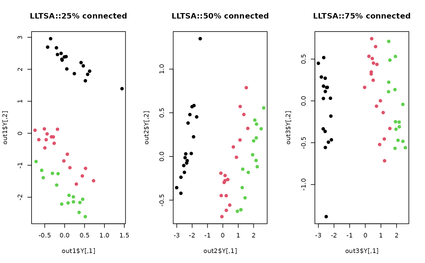
## Visualize three different projections
opar <- par(no.readonly=TRUE)
par(mfrow=c(1,3))
plot(out1$Y, col=lab, pch=19, main="LLTSA::25% connected")
plot(out2$Y, col=lab, pch=19, main="LLTSA::50% connected")
plot(out3$Y, col=lab, pch=19, main="LLTSA::75% connected")

par(opar)