Kernel-Weighted Maximum Variance Projection

Kernel-Weighted Maximum Variance Projection (KMVP) is a generalization of Maximum Variance Projection (MVP). Even though its name contains kernel, it is not related to kernel trick well known in the machine learning community. Rather, it generalizes the binary penalization on class discrepancy, $$S_{ij} = \exp(-\|x_i-x_j\|^2/t) \quad\textrm{if}\quad C_i \ne C_j$$ where $x_i$ is an $i$-th data point and $t$ a kernel bandwidth (bandwidth). Note that when the bandwidth value is too small, it might suffer from numerical instability and rank deficiency due to its formulation.

do.kmvp(
  X,
  label,
  ndim = 2,
  preprocess = c("center", "scale", "cscale", "decorrelate", "whiten"),
  bandwidth = 1
)

Arguments

X: an $(n\times p)$ matrix or data frame whose rows are observations and columns represent independent variables.
label: a length-$n$ vector of data class labels.
ndim: an integer-valued target dimension.
preprocess: an additional option for preprocessing the data. Default is "center". See also aux.preprocess for more details.
bandwidth: bandwidth parameter for heat kernel as the equation above.

Value

a named list containing

Y: an $(n\times ndim)$ matrix whose rows are embedded observations.
trfinfo: a list containing information for out-of-sample prediction.
projection: a $(p\times ndim)$ whose columns are basis for projection.

References

Zhang T (2007). “Maximum Variance Projections for Face Recognition.” Optical Engineering, 46(6), 067206.

Author

Kisung You

Examples

## use iris data
data(iris)
set.seed(100)
subid = sample(1:150, 50)
X     = as.matrix(iris[subid,1:4])
label = as.factor(iris[subid,5])

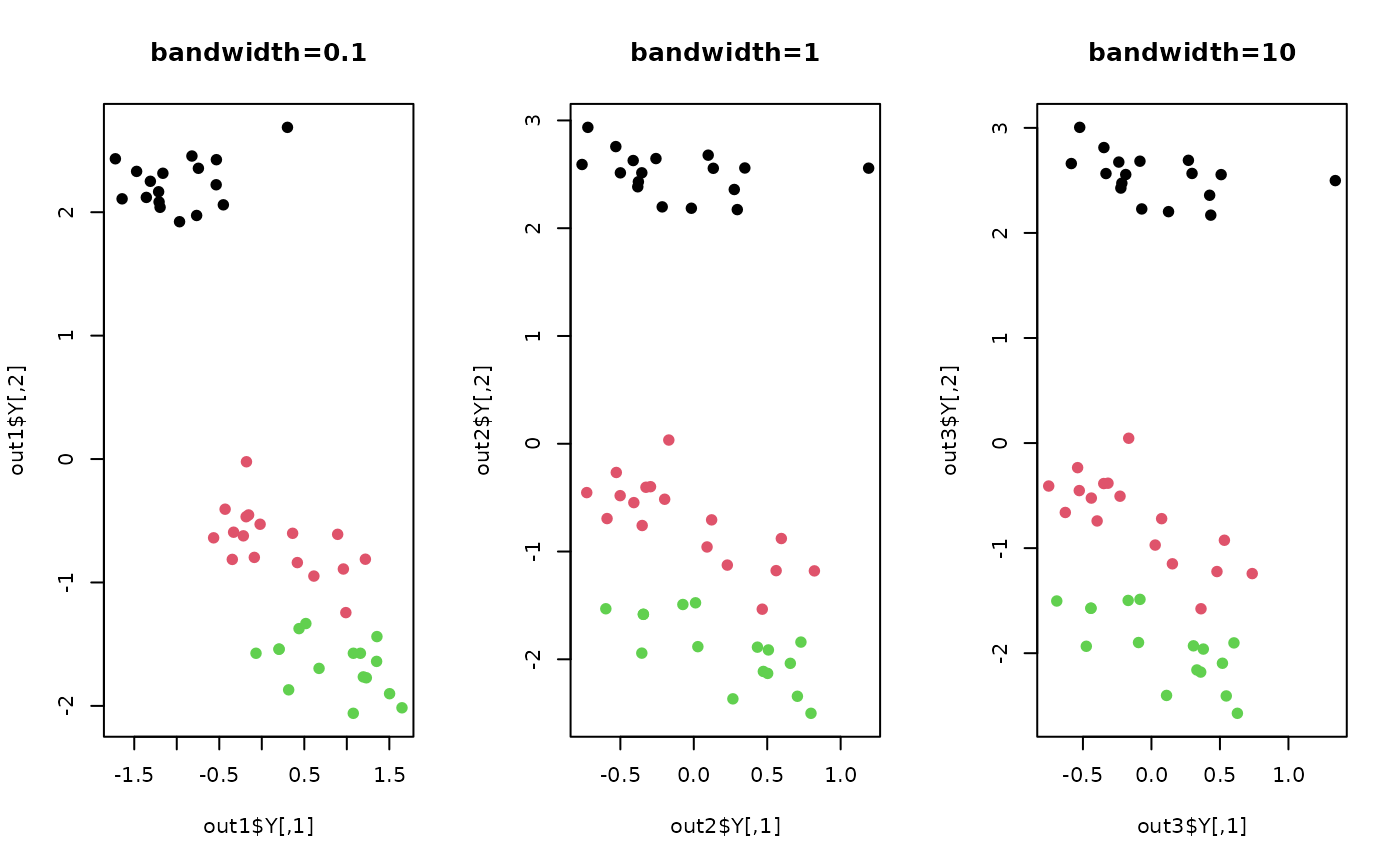
## perform KMVP with different bandwidths
out1 = do.kmvp(X, label, bandwidth=0.1)
out2 = do.kmvp(X, label, bandwidth=1)
out3 = do.kmvp(X, label, bandwidth=10)

## visualize
opar <- par(no.readonly=TRUE)
par(mfrow=c(1,3))
plot(out1$Y, main="bandwidth=0.1", col=label, pch=19)
plot(out2$Y, main="bandwidth=1",   col=label, pch=19)
plot(out3$Y, main="bandwidth=10",  col=label, pch=19)

par(opar)