Isometric Projection

Isometric Projection is a linear dimensionality reduction algorithm that exploits geodesic distance in original data dimension and mimicks the behavior in the target dimension. Embedded manifold is approximated by graph construction as of ISOMAP. Since it involves singular value decomposition and guesses intrinsic dimension by the number of positive singular values from the decomposition of data matrix, it automatically corrects the target dimension accordingly.

do.isoproj(
  X,
  ndim = 2,
  type = c("proportion", 0.1),
  symmetric = c("union", "intersect", "asymmetric"),
  preprocess = c("center", "scale", "cscale", "decorrelate", "whiten")
)

Arguments

X

an \((n\times p)\) matrix or data frame whose rows are observations and columns represent independent variables.

ndim

an integer-valued target dimension.

type

a vector of neighborhood graph construction. Following types are supported; c("knn",k), c("enn",radius), and c("proportion",ratio). Default is c("proportion",0.1), connecting about 1/10 of nearest data points among all data points. See also aux.graphnbd for more details.

symmetric

one of "intersect", "union" or "asymmetric" is supported. Default is "union". See also aux.graphnbd for more details.

preprocess

an additional option for preprocessing the data. Default is "center". See also aux.preprocess for more details.

Value

a named list containing

Y

an \((n\times ndim)\) matrix of projected observations as rows.

projection

a \((p\times ndim)\) whose columns are loadings.

trfinfo

a list containing information for out-of-sample prediction.

References

Cai D, He X, Han J (2007). “Isometric Projection.” In Proceedings of the 22Nd National Conference on Artificial Intelligence - Volume 1, AAAI'07, 528--533. ISBN 978-1-57735-323-2.

Author

Kisung You

Examples

## use iris dataset
data(iris)
set.seed(100)
subid <- sample(1:150, 50)
X     <- as.matrix(iris[subid,1:4])
lab   <- as.factor(iris[subid,5])

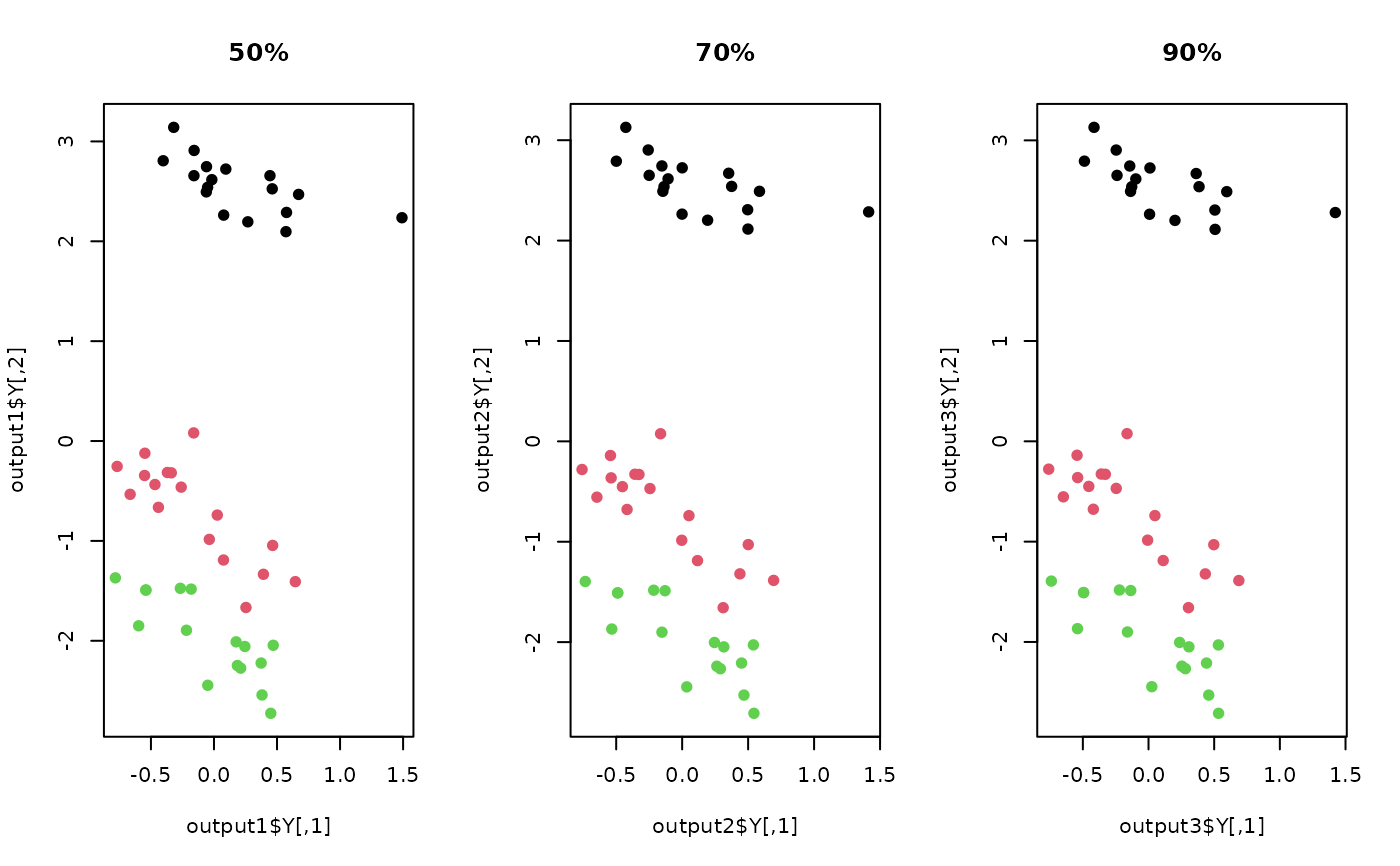
## try different connectivity levels
output1 <- do.isoproj(X,ndim=2,type=c("proportion",0.50))
output2 <- do.isoproj(X,ndim=2,type=c("proportion",0.70))
output3 <- do.isoproj(X,ndim=2,type=c("proportion",0.90))

## visualize two different projections
opar <- par(no.readonly=TRUE)
par(mfrow=c(1,3))
plot(output1$Y, main="50%", col=lab, pch=19)
plot(output2$Y, main="70%", col=lab, pch=19)
plot(output3$Y, main="90%", col=lab, pch=19)

par(opar)