Complete Neighborhood Preserving Embedding

One of drawbacks of Neighborhood Preserving Embedding (NPE) is the small-sample-size problem under high-dimensionality of original data, where singular matrices to be decomposed suffer from rank deficiency. Instead of applying PCA as a preprocessing step, Complete NPE (CNPE) transforms the singular generalized eigensystem computation of NPE into two eigenvalue decomposition problems.

do.cnpe(
  X,
  ndim = 2,
  type = c("proportion", 0.1),
  preprocess = c("center", "scale", "cscale", "decorrelate", "whiten")
)

Arguments

X

an \((n\times p)\) matrix or data frame whose rows are observations and columns represent independent variables.

ndim

an integer-valued target dimension.

type

a vector of neighborhood graph construction. Following types are supported; c("knn",k), c("enn",radius), and c("proportion",ratio). Default is c("proportion",0.1), connecting about 1/10 of nearest data points among all data points. See also aux.graphnbd for more details.

preprocess

an additional option for preprocessing the data. Default is "center". See also aux.preprocess for more details.

Value

a named list containing

Y

an \((n\times ndim)\) matrix whose rows are embedded observations.

trfinfo

a list containing information for out-of-sample prediction.

projection

a \((p\times ndim)\) whose columns are basis for projection.

References

Wang Y, Wu Y (2010). “Complete Neighborhood Preserving Embedding for Face Recognition.” Pattern Recognition, 43(3), 1008--1015.

Author

Kisung You

Examples

# \donttest{
## generate data of 3 types with clear difference
dt1  = aux.gensamples(n=20)-50
dt2  = aux.gensamples(n=20)
dt3  = aux.gensamples(n=20)+50
lab  = rep(1:3, each=20)

## merge the data
X      = rbind(dt1,dt2,dt3)

## try different numbers for neighborhood size
out1 = do.cnpe(X, type=c("proportion",0.10))
out2 = do.cnpe(X, type=c("proportion",0.25))
out3 = do.cnpe(X, type=c("proportion",0.50))

## visualize
opar <- par(no.readonly=TRUE)
par(mfrow=c(1,3))
plot(out1$Y, col=lab, pch=19, main="CNPE::10% connected")
plot(out2$Y, col=lab, pch=19, main="CNPE::25% connected")
plot(out3$Y, col=lab, pch=19, main="CNPE::50% connected")

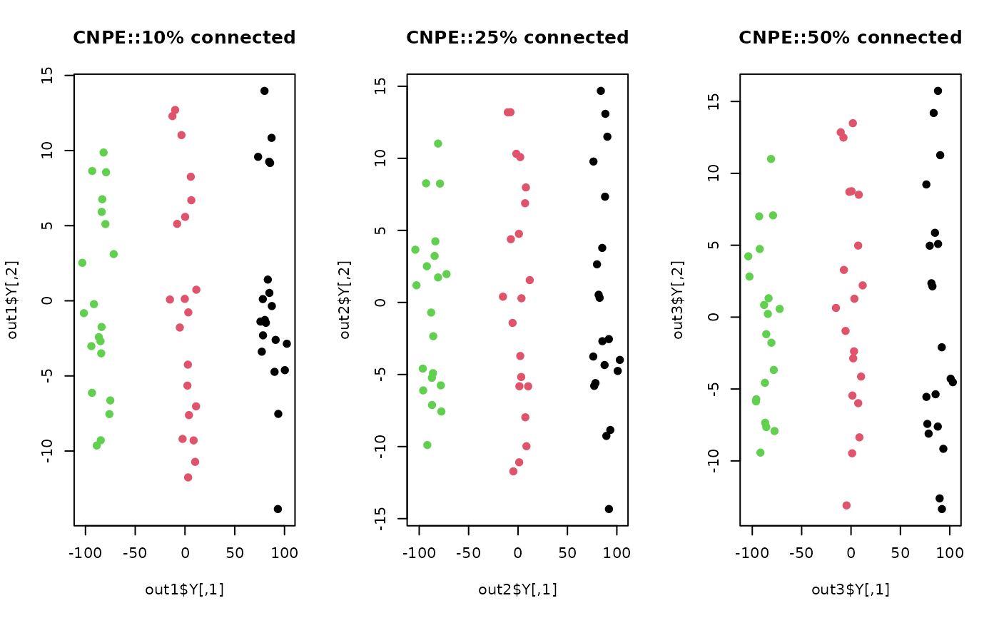par(opar)
# }