Multi-Cluster Feature Selection — do.mcfs • Rdimtools

Multi-Cluster Feature Selection (MCFS) is an unsupervised feature selection method. Based on a multi-cluster assumption, it aims at finding meaningful features using sparse reconstruction of spectral basis using LASSO.

do.mcfs(
  X,
  ndim = 2,
  type = c("proportion", 0.1),
  preprocess = c("null", "center", "scale", "cscale", "whiten", "decorrelate"),
  K = max(round(nrow(X)/5), 2),
  lambda = 1,
  t = 10
)

Arguments

X: an \((n\times p)\) matrix or data frame whose rows are observations and columns represent independent variables.
ndim: an integer-valued target dimension.
type: a vector of neighborhood graph construction. Following types are supported; c("knn",k), c("enn",radius), and c("proportion",ratio). Default is c("proportion",0.1), connecting about 1/10 of nearest data points among all data points. See also aux.graphnbd for more details.
preprocess: an additional option for preprocessing the data. Default is "null". See also aux.preprocess for more details.
K: assumed number of clusters in the original dataset.
lambda: \(\ell_1\) regularization parameter in \((0,\infty)\).
t: bandwidth parameter for heat kernel in \((0,\infty)\).

Value

a named list containing

Y: an \((n\times ndim)\) matrix whose rows are embedded observations.
featidx: a length-\(ndim\) vector of indices with highest scores.
trfinfo: a list containing information for out-of-sample prediction.
projection: a \((p\times ndim)\) whose columns are basis for projection.

References

Cai D, Zhang C, He X (2010). “Unsupervised Feature Selection for Multi-Cluster Data.” In Proceedings of the 16th ACM SIGKDD International Conference on Knowledge Discovery and Data Mining, 333--342.

Author

Kisung You

Examples

## generate data of 3 types with clear difference
dt1  = aux.gensamples(n=20)-100
dt2  = aux.gensamples(n=20)
dt3  = aux.gensamples(n=20)+100

## merge the data and create a label correspondingly
X      = rbind(dt1,dt2,dt3)
label  = rep(1:3, each=20)

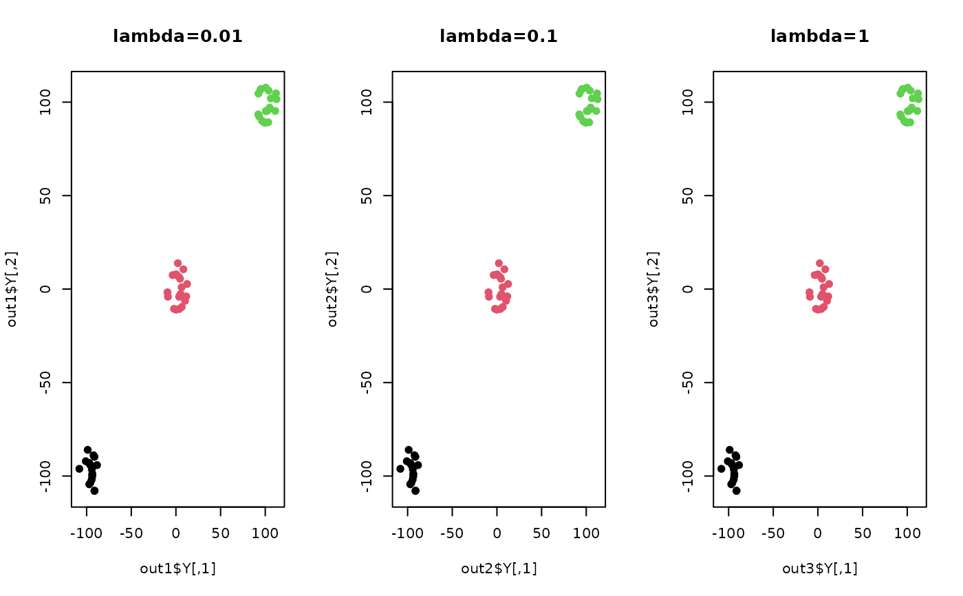
## try different regularization parameters
out1 = do.mcfs(X, lambda=0.01)
out2 = do.mcfs(X, lambda=0.1)
out3 = do.mcfs(X, lambda=1)

## visualize
opar <- par(no.readonly=TRUE)
par(mfrow=c(1,3))
plot(out1$Y, pch=19, col=label, main="lambda=0.01")
plot(out2$Y, pch=19, col=label, main="lambda=0.1")
plot(out3$Y, pch=19, col=label, main="lambda=1")

par(opar)