Spectral Clustering by Yang et al. (2011)

As a data-driven method, the algorithm recovers geodesic distance from a k-nearest neighbor graph scaled by an (exponential) parameter \(\rho\) and applies random-walk spectral clustering. Authors referred their method as density sensitive similarity function.

sc11Y(data, k = 2, nnbd = 7, rho = 2, ...)

Arguments

data	an \((n\times p)\) matrix of row-stacked observations or S3 dist object of \(n\) observations.
k	the number of clusters (default: 2).
nnbd	neighborhood size to define data-driven bandwidth parameter (default: 7).
rho	exponent scaling parameter (default: 2).
...	extra parameters including algclust method to perform clustering on embedded data; either "kmeans" (default) or "GMM". maxiter the maximum number of iterations (default: 10).

Value

a named list of S3 class T4cluster containing

cluster

a length-\(n\) vector of class labels (from \(1:k\)).

eigval

eigenvalues of the graph laplacian's spectral decomposition.

embeds

an \((n\times k)\) low-dimensional embedding.

algorithm

name of the algorithm.

References

Yang P, Zhu Q, Huang B (2011). “Spectral Clustering with Density Sensitive Similarity Function.” Knowledge-Based Systems, 24(5), 621--628. ISSN 09507051.

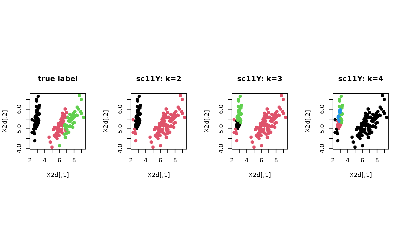
Examples

# -------------------------------------------------------------
#            clustering with 'iris' dataset
# -------------------------------------------------------------
## PREPARE
data(iris)
X   = as.matrix(iris[,1:4])
lab = as.integer(as.factor(iris[,5]))

## EMBEDDING WITH PCA
X2d = Rdimtools::do.pca(X, ndim=2)$Y

## CLUSTERING WITH DIFFERENT K VALUES
cl2 = sc11Y(X, k=2)$cluster
cl3 = sc11Y(X, k=3)$cluster
cl4 = sc11Y(X, k=4)$cluster

## VISUALIZATION
opar <- par(no.readonly=TRUE)
par(mfrow=c(1,4), pty="s")
plot(X2d, col=lab, pch=19, main="true label")
plot(X2d, col=cl2, pch=19, main="sc11Y: k=2")
plot(X2d, col=cl3, pch=19, main="sc11Y: k=3")
plot(X2d, col=cl4, pch=19, main="sc11Y: k=4")
par(opar)