Spectral Clustering by Zhang et al. (2010)

The algorithm defines a set of data-driven bandwidth parameters \(p_{ij}\) by constructing a similarity matrix. Then the affinity matrix is defined as $$A_{ij} = \exp(-d(x_i, d_j)^2 / 2 p_{ij})$$ and the standard spectral clustering of Ng, Jordan, and Weiss (scNJW) is applied.

sc10Z(data, k = 2, ...)

Arguments

data	an \((n\times p)\) matrix of row-stacked observations or S3 dist object of \(n\) observations.
k	the number of clusters (default: 2).
...	extra parameters including algclust method to perform clustering on embedded data; either "kmeans" (default) or "GMM". maxiter the maximum number of iterations (default: 10).

Value

a named list of S3 class T4cluster containing

cluster

a length-\(n\) vector of class labels (from \(1:k\)).

eigval

eigenvalues of the graph laplacian's spectral decomposition.

embeds

an \((n\times k)\) low-dimensional embedding.

algorithm

name of the algorithm.

References

Zhang Y, Zhou J, Fu Y (2010). “Spectral Clustering Algorithm Based on Adaptive Neighbor Distance Sort Order.” In The 3rd International Conference on Information Sciences and Interaction Sciences, 444--447. ISBN 978-1-4244-7384-7.

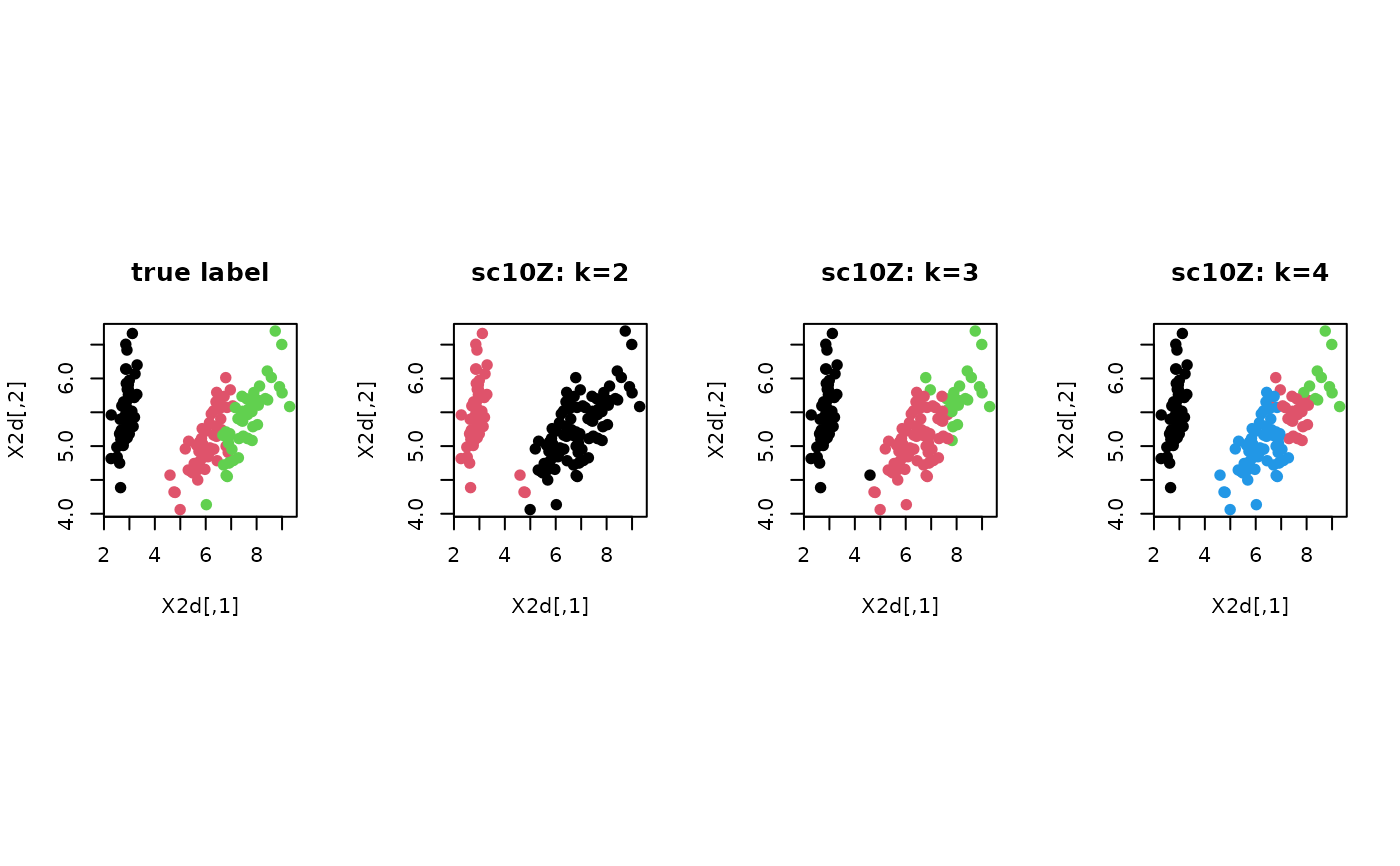
Examples

# -------------------------------------------------------------
#            clustering with 'iris' dataset
# -------------------------------------------------------------
## PREPARE
data(iris)
X   = as.matrix(iris[,1:4])
lab = as.integer(as.factor(iris[,5]))

## EMBEDDING WITH PCA
X2d = Rdimtools::do.pca(X, ndim=2)$Y

## CLUSTERING WITH DIFFERENT K VALUES
cl2 = sc10Z(X, k=2)$cluster
cl3 = sc10Z(X, k=3)$cluster
cl4 = sc10Z(X, k=4)$cluster

## VISUALIZATION
opar <- par(no.readonly=TRUE)
par(mfrow=c(1,4), pty="s")
plot(X2d, col=lab, pch=19, main="true label")
plot(X2d, col=cl2, pch=19, main="sc10Z: k=2")
plot(X2d, col=cl3, pch=19, main="sc10Z: k=3")
plot(X2d, col=cl4, pch=19, main="sc10Z: k=4")
par(opar)