Spectral Clustering by Gu and Wang (2009)

The algorithm defines a set of data-driven bandwidth parameters where $\sigma_i$ is the average distance from a point $x_i$ to its nnbd-th nearest neighbor. Then the affinity matrix is defined as $$A_{ij} = \exp(-d(x_i, d_j)^2 / \sigma_i \sigma_j)$$ and the standard spectral clustering of Ng, Jordan, and Weiss (scNJW) is applied.

sc09G(data, k = 2, nnbd = 7, ...)

Arguments

data	an $(n\times p)$ matrix of row-stacked observations or S3 `dist` object of $n$ observations.
k	the number of clusters (default: 2).
nnbd	neighborhood size to define data-driven bandwidth parameter (default: 7).
...	extra parameters including algclust method to perform clustering on embedded data; either `"kmeans"` (default) or `"GMM"`. maxiter the maximum number of iterations (default: 10).

Value

a named list of S3 class T4cluster containing

cluster: a length-$n$ vector of class labels (from $1:k$).
eigval: eigenvalues of the graph laplacian's spectral decomposition.
embeds: an $(n\times k)$ low-dimensional embedding.
algorithm: name of the algorithm.

References

Gu R, Wang J (2009). “An Improved Spectral Clustering Algorithm Based on Neighbour Adaptive Scale.” In 2009 International Conference on Business Intelligence and Financial Engineering, 233--236. ISBN 978-0-7695-3705-4.

Examples

# -------------------------------------------------------------
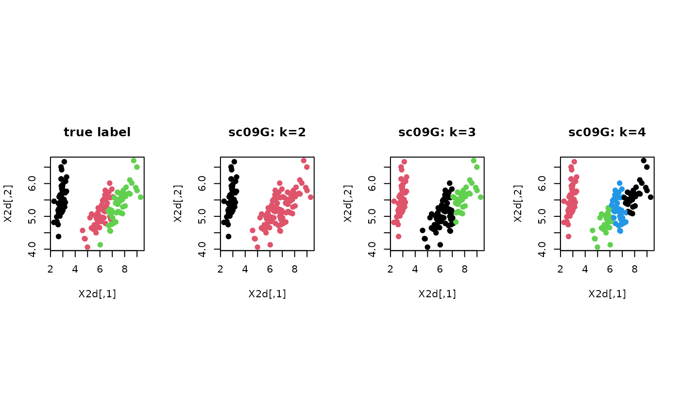
#            clustering with 'iris' dataset
# -------------------------------------------------------------
## PREPARE
data(iris)
X   = as.matrix(iris[,1:4])
lab = as.integer(as.factor(iris[,5]))

## EMBEDDING WITH PCA
X2d = Rdimtools::do.pca(X, ndim=2)$Y

## CLUSTERING WITH DIFFERENT K VALUES
cl2 = sc09G(X, k=2)$cluster
cl3 = sc09G(X, k=3)$cluster
cl4 = sc09G(X, k=4)$cluster

## VISUALIZATION
opar <- par(no.readonly=TRUE)
par(mfrow=c(1,4), pty="s")
plot(X2d, col=lab, pch=19, main="true label")
plot(X2d, col=cl2, pch=19, main="sc09G: k=2")
plot(X2d, col=cl3, pch=19, main="sc09G: k=3")
plot(X2d, col=cl4, pch=19, main="sc09G: k=4")
par(opar)

data	an \((n\times p)\) matrix of row-stacked observations or S3 `dist` object of \(n\) observations.
k	the number of clusters (default: 2).
nnbd	neighborhood size to define data-driven bandwidth parameter (default: 7).
...	extra parameters including algclust method to perform clustering on embedded data; either `"kmeans"` (default) or `"GMM"`. maxiter the maximum number of iterations (default: 10).