Apply \(k\)-means clustering algorithm on top of the lightweight coreset as proposed in the paper. The smaller the set is, the faster the execution becomes with potentially larger quantization errors.
kmeans18B(data, k = 2, m = round(nrow(data)/2), ...)
Arguments
| data | an \((n\times p)\) matrix of row-stacked observations. |
|---|---|
| k | the number of clusters (default: 2). |
| m | the size of coreset (default: \(n/2\)). |
| ... | extra parameters including
|
Value
a named list of S3 class T4cluster containing
- cluster
a length-\(n\) vector of class labels (from \(1:k\)).
- mean
a \((k\times p)\) matrix where each row is a class mean.
- wcss
within-cluster sum of squares (WCSS).
- algorithm
name of the algorithm.
References
Bachem O, Lucic M, Krause A (2018). “Scalable k -Means Clustering via Lightweight Coresets.” In Proceedings of the 24th ACM SIGKDD International Conference on Knowledge Discovery \& Data Mining, 1119--1127. ISBN 978-1-4503-5552-0.
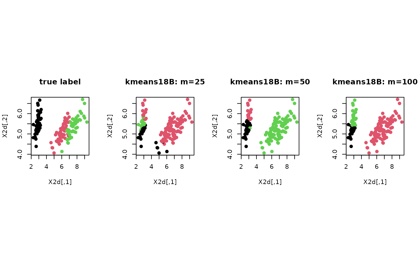
Examples
# ------------------------------------------------------------- # clustering with 'iris' dataset # ------------------------------------------------------------- ## PREPARE data(iris) X = as.matrix(iris[,1:4]) lab = as.integer(as.factor(iris[,5])) ## EMBEDDING WITH PCA X2d = Rdimtools::do.pca(X, ndim=2)$Y ## CLUSTERING WITH DIFFERENT CORESET SIZES WITH K=3 core1 = kmeans18B(X, k=3, m=25)$cluster core2 = kmeans18B(X, k=3, m=50)$cluster core3 = kmeans18B(X, k=3, m=100)$cluster ## VISUALIZATION opar <- par(no.readonly=TRUE) par(mfrow=c(1,4), pty="s") plot(X2d, col=lab, pch=19, main="true label") plot(X2d, col=core1, pch=19, main="kmeans18B: m=25") plot(X2d, col=core2, pch=19, main="kmeans18B: m=50") plot(X2d, col=core3, pch=19, main="kmeans18B: m=100")