Finite Gaussian Mixture Model (GMM) is a well-known probabilistic clustering algorithm by fitting the following distribution to the data $$f(x; \left\lbrace \mu_k, \Sigma_k \right\rbrace_{k=1}^K) = \sum_{k=1}^K w_k N(x; \mu_k, \Sigma_k)$$ with parameters \(w_k\)'s for cluster weights, \(\mu_k\)'s for class means, and \(\Sigma_k\)'s for class covariances. This function is a wrapper for Armadillo's GMM function, which supports two types of covariance models.
gmm(data, k = 2, ...)
Arguments
| data | an \((n\times p)\) matrix of row-stacked observations. |
|---|---|
| k | the number of clusters (default: 2). |
| ... | extra parameters including
|
Value
a named list of S3 class T4cluster containing
- cluster
a length-\(n\) vector of class labels (from \(1:k\)).
- mean
a \((k\times p)\) matrix where each row is a class mean.
- variance
a \((p\times p\times k)\) array where each slice is a class covariance.
- weight
a length-\(k\) vector of class weights that sum to 1.
- loglkd
log-likelihood of the data for the fitted model.
- algorithm
name of the algorithm.
Examples
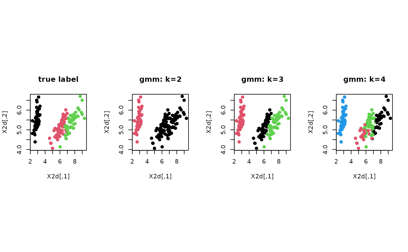
# ------------------------------------------------------------- # clustering with 'iris' dataset # ------------------------------------------------------------- ## PREPARE data(iris) X = as.matrix(iris[,1:4]) lab = as.integer(as.factor(iris[,5])) ## EMBEDDING WITH PCA X2d = Rdimtools::do.pca(X, ndim=2)$Y ## CLUSTERING WITH DIFFERENT K VALUES cl2 = gmm(X, k=2)$cluster cl3 = gmm(X, k=3)$cluster cl4 = gmm(X, k=4)$cluster ## VISUALIZATION opar <- par(no.readonly=TRUE) par(mfrow=c(1,4), pty="s") plot(X2d, col=lab, pch=19, main="true label") plot(X2d, col=cl2, pch=19, main="gmm: k=2") plot(X2d, col=cl3, pch=19, main="gmm: k=3") plot(X2d, col=cl4, pch=19, main="gmm: k=4")
