Functional Hierarchical Clustering

Given \(N\) curves \(\gamma_1 (t), \gamma_2 (t), \ldots, \gamma_N (t) : I \rightarrow \mathbf{R}\), perform hierarchical agglomerative clustering with fastcluster package's implementation of the algorithm. Dissimilarity for curves is measured by \(L_p\) metric.

funhclust(
  fdobj,
  p = 2,
  method = c("single", "complete", "average", "mcquitty", "ward.D", "ward.D2",
    "centroid", "median"),
  members = NULL
)

Arguments

fdobj	a 'fd' functional data object of \(N\) curves by the fda package.
p	an exponent in \(L_p\) formalism (default: 2).
method	agglomeration method to be used. This must be one of "single", "complete", "average", "mcquitty", "ward.D", "ward.D2", "centroid" or "median".
members	NULL or a vector whose length equals the number of observations. See hclust for details.

Value

an object of class hclust. See hclust for details.

References

Ferreira L, Hitchcock DB (2009). “A Comparison of Hierarchical Methods for Clustering Functional Data.” Communications in Statistics - Simulation and Computation, 38(9), 1925--1949. ISSN 0361-0918, 1532-4141.

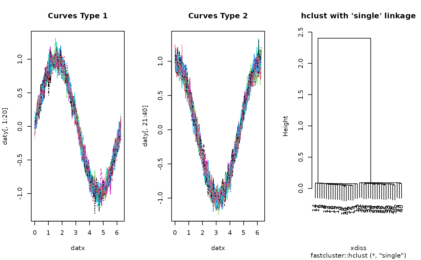
Examples

# -------------------------------------------------------------
#                     two types of curves
#
# type 1 : sin(x) + perturbation; 20 OF THESE ON [0, 2*PI]
# type 2 : cos(x) + perturbation; 20 OF THESE ON [0, 2*PI]
# -------------------------------------------------------------
## PREPARE : USE 'fda' PACKAGE
#  Generate Raw Data
datx = seq(from=0, to=2*pi, length.out=100)
daty = array(0,c(100, 40))
for (i in 1:20){
  daty[,i]    = sin(datx) + rnorm(100, sd=0.1)
  daty[,i+20] = cos(datx) + rnorm(100, sd=0.1)
}
#  Wrap as 'fd' object
mybasis <- fda::create.bspline.basis(c(0,2*pi), nbasis=10)
myfdobj <- fda::smooth.basis(datx, daty, mybasis)$fd

## RUN THE ALGORITHM 
hcsingle = funhclust(myfdobj, method="single")

## VISUALIZE
opar <- par(no.readonly=TRUE)
par(mfrow=c(1,3))
matplot(datx, daty[,1:20],  type="l", main="Curves Type 1")
matplot(datx, daty[,21:40], type="l", main="Curves Type 2")
plot(hcsingle, main="hclust with 'single' linkage")
par(opar)