Stochastic Neighbor Embedding

Stochastic Neighbor Embedding (SNE) is a probabilistic approach to mimick distributional description in high-dimensional - possible, nonlinear - subspace on low-dimensional target space. do.sne fully adopts algorithm details in an original paper by Hinton and Roweis (2002).

do.sne(
  X,
  ndim = 2,
  perplexity = 30,
  eta = 0.05,
  maxiter = 2000,
  jitter = 0.3,
  jitterdecay = 0.99,
  momentum = 0.5,
  pca = TRUE,
  pcascale = FALSE,
  symmetric = FALSE
)

Arguments

X

an \((n\times p)\) matrix or data frame whose rows are observations and columns represent independent variables.

ndim

an integer-valued target dimension.

perplexity

desired level of perplexity; ranging [5,50].

eta

learning parameter.

maxiter

maximum number of iterations.

jitter

level of white noise added at the beginning.

jitterdecay

decay parameter in \((0,1)\). The closer to 0, the faster artificial noise decays.

momentum

level of acceleration in learning.

pca

whether to use PCA as preliminary step; TRUE for using it, FALSE otherwise.

pcascale

a logical; FALSE for using Covariance, TRUE for using Correlation matrix. See also do.pca for more details.

symmetric

a logical; FALSE to solve it naively, and TRUE to adopt symmetrization scheme.

Value

a named Rdimtools S3 object containing

Y

an \((n\times ndim)\) matrix whose rows are embedded observations.

vars

a vector containing betas used in perplexity matching.

algorithm

name of the algorithm.

References

Hinton GE, Roweis ST (2003). “Stochastic Neighbor Embedding.” In Becker S, Thrun S, Obermayer K (eds.), Advances in Neural Information Processing Systems 15, 857--864. MIT Press.

Author

Kisung You

Examples

# \donttest{
## load iris data
data(iris)
set.seed(100)
subid = sample(1:150,50)
X     = as.matrix(iris[subid,1:4])
label = as.factor(iris[subid,5])

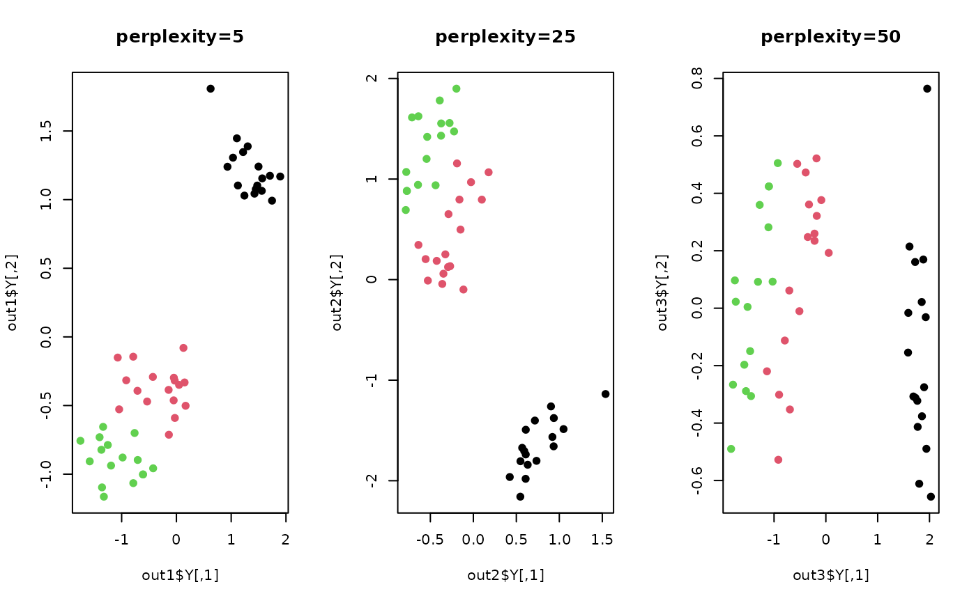
## try different perplexity values
out1 <- do.sne(X, perplexity=5)
out2 <- do.sne(X, perplexity=25)
out3 <- do.sne(X, perplexity=50)

## Visualize two comparisons
opar <- par(no.readonly=TRUE)
par(mfrow=c(1,3))
plot(out1$Y, pch=19, col=label, main="perplexity=5")
plot(out2$Y, pch=19, col=label, main="perplexity=25")
plot(out3$Y, pch=19, col=label, main="perplexity=50")

par(opar)
# }