Metric MDS is a nonlinear method that is solved iteratively. We adopt a well-known SMACOF algorithm for updates with uniform weights over all pairwise distances after initializing the low-dimensional configuration via classical MDS.
do.mmds(X, ndim = 2, ...)Arguments
- X
an \((n\times p)\) matrix or data frame whose rows are observations and columns represent independent variables.
- ndim
an integer-valued target dimension (default: 2).
- ...
extra parameters including
- maxiter
maximum number of iterations for metric MDS updates (default: 100).
- abstol
stopping criterion for metric MDS iterations (default: 1e-8).
Value
a named Rdimtools S3 object containing
- Y
an \((n\times ndim)\) matrix whose rows are embedded observations.
- algorithm
name of the algorithm.
References
Leeuw JD, Barra IJR, Brodeau F, Romier G, (eds BVC (1977). “Applications of Convex Analysis to Multidimensional Scaling.” In Recent Developments in Statistics, 133–146.
Borg I, Groenen PJF (2010). Modern Multidimensional Scaling: Theory and Applications. Springer New York, New York, NY. ISBN 978-1-4419-2046-1 978-0-387-28981-6.
Examples
# \donttest{
## load iris data
data(iris)
X = as.matrix(iris[,1:4])
lab = as.factor(iris[,5])
## compare with other methods
pca2d <- do.pca(X, ndim=2)
cmd2d <- do.mds(X, ndim=2)
mmd2d <- do.mmds(X, ndim=2)
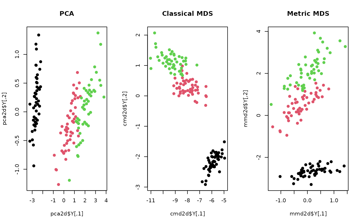
## Visualize
opar <- par(no.readonly=TRUE)
par(mfrow=c(1,3))
plot(pca2d$Y, col=lab, pch=19, main="PCA")
plot(cmd2d$Y, col=lab, pch=19, main="Classical MDS")
plot(mmd2d$Y, col=lab, pch=19, main="Metric MDS")
 par(opar)
# }
par(opar)
# }